Cell State Transition Analysis with scMagnify#
Preliminaries#
scMagnify is a versatile Python toolkit for inferring and analyzing gene regulatory networks (GRNs) from single-cell multi-omic datasets.
In this tutorial, you will learn how to:
Fate Mapping. Use
cellrank[LBK+22, WLK+24] to infer fate probabilities and construct a transition matrix of cellular dynamics.Cell State Selection. Perform lineage classifer or paga graph operator to select cell state you are interested in.
Feature Association Test. Annotate significantly changing feature along pseudotime test.
Note
This tutorial aims to assist users in preprocessing the scRNAseq data for scMagnify analysis. cellrank is a unified fate-mapping framework designed for studying cellular dynamics through Markov state modeling of multi-view single-cell data. For detailed instructions on the usage of cellrank, please refer to the official tutorial.
And this tutorial does not cover the preprocessing of scRNA-seq data, nor the computation of pseudotime or RNA velocity. Please refer to the relevant documentation for those topics:
Import packages#
%load_ext autoreload
%autoreload 2
import warnings
from numba.core.errors import NumbaDeprecationWarning

warnings.simplefilter("ignore", category=NumbaDeprecationWarning)
warnings.simplefilter("ignore", FutureWarning)
warnings.simplefilter("ignore", UserWarning)
warnings.simplefilter("ignore", RuntimeWarning)
import os
import pandas as pd

import matplotlib.pyplot as plt
import scanpy as sc
import cellrank as cr
import scmagnify as scm
from scmagnify.settings import settings
scm.info()
 |
|
Configurations#
Before starting the analysis, we need to configure our environment. This primarily involves four steps:
Downloading built-in data
Initializing plot settings
Setting a workspace
Specifying a reference genome
First, if you are using scMagnify for the first time, please run the following command to fetch the required annotations. This only needs to be performed once.
scm.settings.verbosity = 2
os.environ["SCMAGNIFY_DATA"] = "/mnt/TrueNas/project/chenxufeng/Caches/scmagnify/"
scm.datasets.fetch_scm_data()
INFO     Moving from '/mnt/TrueNas/project/chenxufeng/Caches/scmagnify/scmagnify_data.zip.unzip/data' to
         '/mnt/TrueNas/project/chenxufeng/Caches/scmagnify/scm_data'...
INFO Cleaned up temporary directory: /mnt/TrueNas/project/chenxufeng/Caches/scmagnify/scmagnify_data.zip.unzip
INFO     Could not clean up temporary directory
         /mnt/TrueNas/project/chenxufeng/Caches/scmagnify/scmagnify_data.zip.unzip: [Errno 20] Not a directory:
         '/mnt/TrueNas/project/chenxufeng/Caches/scmagnify/scmagnify_data.zip'
'/mnt/TrueNas/project/chenxufeng/Caches/scmagnify/scm_data'
Note
scMagnify uses pooch to manage built-in datasets. By default, all data is cached in the ./caches/scmagnify/. If you wish to change this location, you can set the SCMAGNIFY_DATA environment variable.
For more details on data management, please see [Advanced Usages/Configurations](./Advanced Usages/Configurations.md) and the official pooch documentation. :::
Now, let’s proceed with the other configuration steps.
%matplotlib inline

scm.settings.set_figure_params(
    dpi=100,
    facecolor="white",
    frameon=False,
)

# Load fonts from scm_data
scm.load_fonts(["Arial"])

plt.rcParams["font.family"] = "Arial"
plt.rcParams["grid.alpha"] = 0
plt.rcParams["savefig.dpi"] = 300
# Setting a workspace
dirPjtHome = "/mnt/TrueNas/project/chenxufeng/Data/PMID36973557_NatBiotechnol2023_T-cell-depleted/"
workDir = os.path.join(dirPjtHome, "scmagnify_wd")
scm.set_workspace(workDir)
workspace: /mnt/TrueNas/project/chenxufeng/Data/PMID36973557_NatBiotechnol2023_T-cell-depleted/scmagnify_wd/
├── data
├── models
├── tmpfiles
└── figures
# Set up Reference Genome
scm.set_genome(version="hg38", genomes_dir="/home/chenxufeng/picb_cxf/Ref/human/hg38/")
                        Genome Information
┏━━━━━━━━━┳━━━━━━━━━━┳━━━━━━━━━━━━━━━━━━━━━━━━━━━━━━━━━━━━━━━━━━━┓
┃ Version ┃ Provider ┃ Directory                                 ┃
┡━━━━━━━━━╇━━━━━━━━━━╇━━━━━━━━━━━━━━━━━━━━━━━━━━━━━━━━━━━━━━━━━━━┩
│ hg38    │ UCSC     │ /home/chenxufeng/picb_cxf/Ref/human/hg38/ │
└─────────┴──────────┴───────────────────────────────────────────┘
Note
scMagnify utilizes genompy{cite}`` for managing reference genome files. genompy simplifies the process of searching, downloading, and preprocessing genomes and annotations from providers like UCSC, Ensembl, and GENCODE.
For more details on managing genome files, please see [Advanced Usages/Configurations](./Advanced Usages/Configurations.md) and the official genompy documentation. :::
Load the data#
To demonstrate the approach in this tutorial, we will use a human blood dataset containing single-cell multi-omic data of CD34+ bone marrow cells from healthy donors, which can be conveniently acessed through human_tcelldep_bm {cite}.
Since we have already configured a workspace, the dataset will be automatically downloaded and stored in scm.settings.data_dir.
mdata = scm.datasets.human_tcelldep_bm()
mdata = scm.read(os.path.join(settings.data_dir, "mdata_tcelldep-bm_raw.h5mu"))
mdata
MuData object with n_obs × n_vars = 8627 × 233703
2 modalities
ATAC: 8627 x 216477
obs: 'sample', 'celltype', 'TSSEnrichment', 'NucleosomeRatio', 'nFrags', 'BlacklistRatio'
var: 'seqnames', 'start', 'end', 'strand', 'GC', 'Bcells_primed', 'Bcells_lineage_specific'
uns: 'celltype_colors', 'neighbors', 'sample_colors', 'umap'
obsm: 'DM_EigenVectors', 'GeneScores', 'X_svd', 'X_umap'
layers: 'counts'
obsp: 'connectivities', 'distances'
RNA: 8627 x 17226
obs: 'sample', 'celltype', 'palantir_pseudotime'
var: 'highly_variable'
uns: 'celltype_colors', 'neighbors', 'sample_colors', 'umap'
obsm: 'X_FDL', 'X_pca', 'X_umap'
layers: 'MAGIC_imputed_data', 'counts'
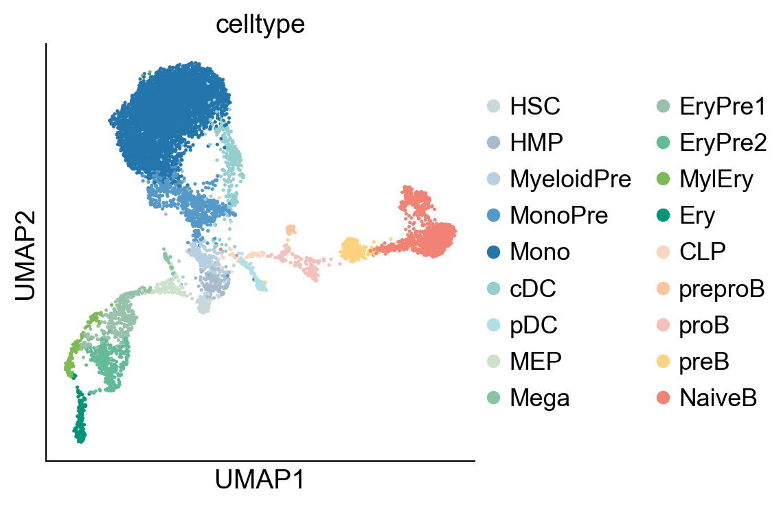
obsp: 'connectivities', 'distances', 'knn'adata = mdata["RNA"]
sc.pl.umap(adata, color=["celltype"])
Fate mapping with CellRank#
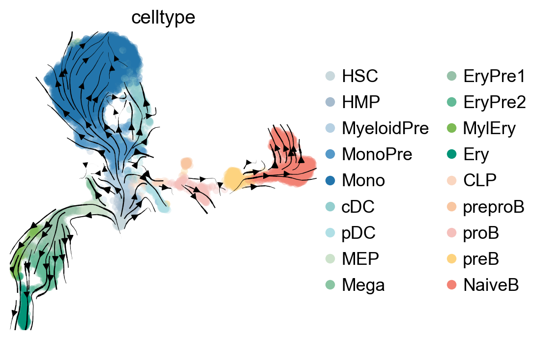
pk = cr.kernels.PseudotimeKernel(adata, time_key="palantir_pseudotime")
pk.compute_transition_matrix()
PseudotimeKernel[n=8627, dnorm=False, scheme='hard', frac_to_keep=0.3]
pk.plot_projection(basis="umap", recompute=True, color="celltype", legend_loc="right")
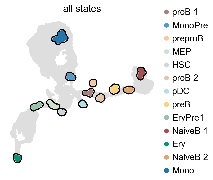
g = cr.estimators.GPCCA(pk)
g.compute_macrostates(n_states=13, cluster_key="celltype")
g.plot_macrostates(which="all", discrete=True, legend_loc="right", s=100)
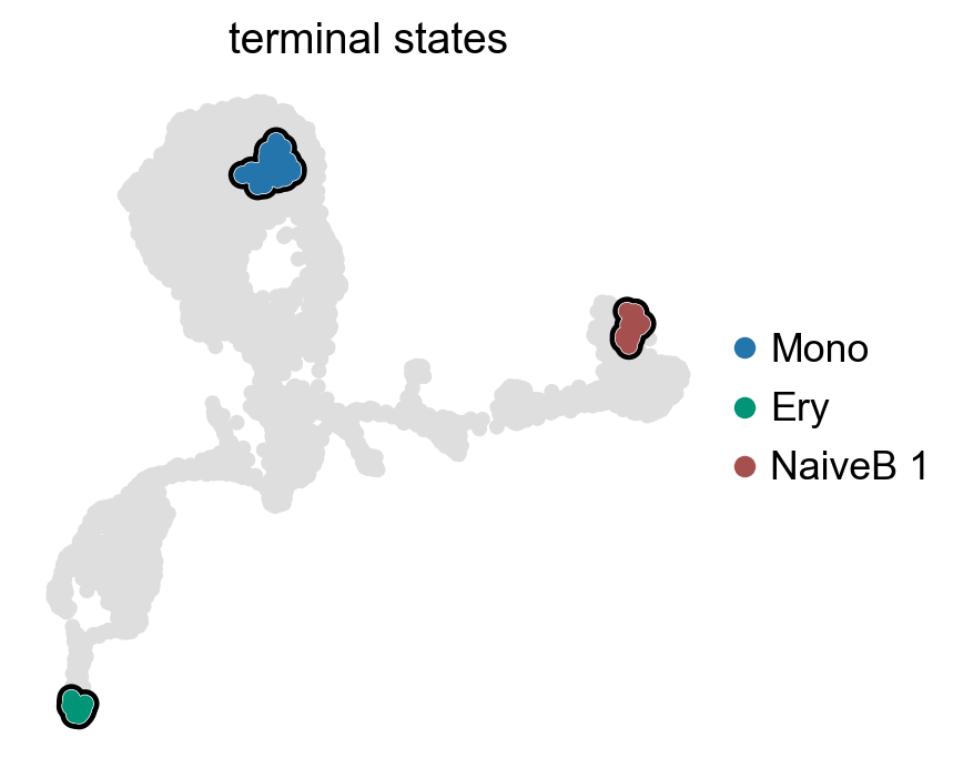
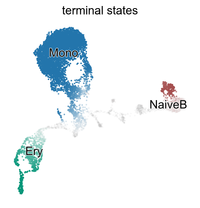
g.set_terminal_states(states=["Mono", "Ery", "NaiveB_1"])
g.plot_macrostates(which="terminal", legend_loc="right", s=100)
g.rename_terminal_states({"NaiveB_1": "NaiveB"})
g.plot_macrostates(which="terminal", discrete=False)
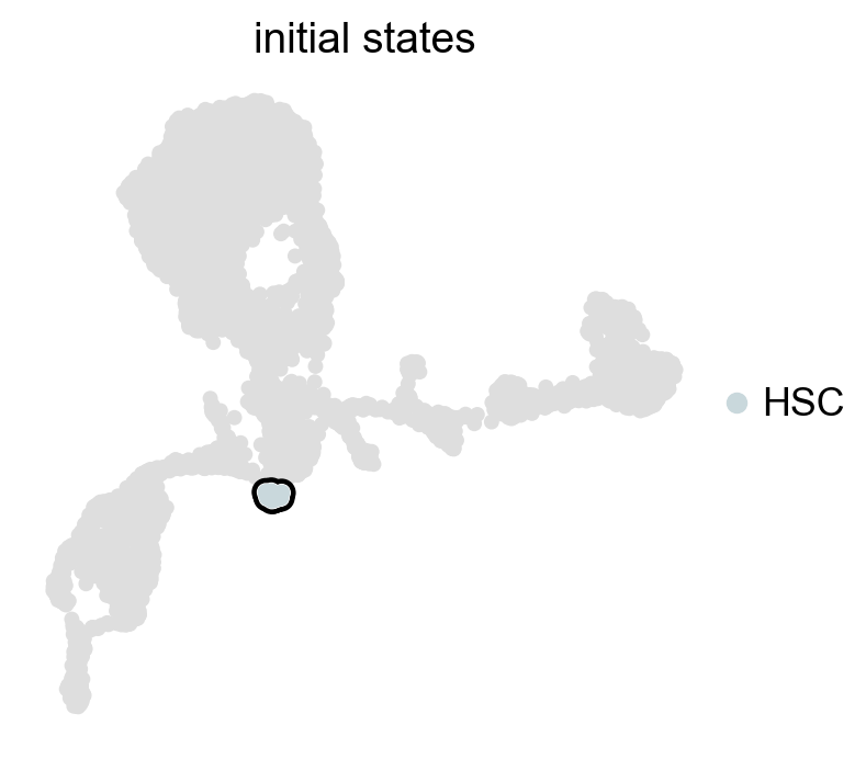
g.set_initial_states(states=["HSC"])
g.plot_macrostates(which="initial", legend_loc="right", s=100)
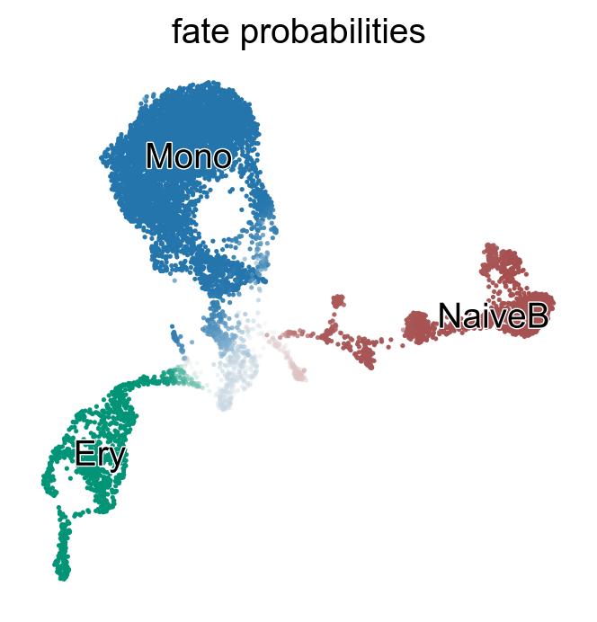
g.compute_fate_probabilities()
g.plot_fate_probabilities(same_plot=True)
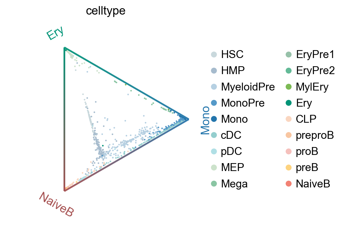
cr.pl.circular_projection(adata, keys=["celltype"], legend_loc="right")
adata.obsm["cellrank_fate_probabilities"] = pd.DataFrame(
    g.fate_probabilities, index=adata.obs_names, columns=g.terminal_states.cat.categories
)
Selecting by Lineage Classifer#
Now that we have stored the cellrank_fate_probabilities in adata.obsm, we can use these probabilities to formally classify cells into their most likely lineage. This provides a clear-cut assignment for selecting cells belonging to a specific fate.
mdata = scm.tl.lineage_classifer(mdata)
INFO .obsm['cell_state_masks'] --> added
       Cell State Statistics
┏━━━━━━━━━━━━┳━━━━━━━━┳━━━━━━━━━━━━┓
┃ Cell State ┃ Number ┃ Percentage ┃
┡━━━━━━━━━━━━╇━━━━━━━━╇━━━━━━━━━━━━┩
│    Mono    │  5556  │   64.40%   │
│    Ery     │  993   │   11.51%   │
│   NaiveB   │  1379  │   15.98%   │
└────────────┴────────┴────────────┘
INFO     Saved masks in
         /mnt/TrueNas/project/chenxufeng/Data/PMID36973557_NatBiotechnol2023_T-cell-depleted/scmagnify_wd/tmpfiles/
         cell_state_masks.csv
Warning
You should manually remove cell types from the lineage that contradict established biological knowledge.
for lineage in adata.obsm["cell_state_masks"].columns:
    print(adata[adata.obsm["cell_state_masks"][lineage]].obs.celltype.value_counts())
celltype
Mono          4659
MonoPre        607
cDC            131
MyeloidPre      88
HSC             38
HMP             32
pDC              1
Name: count, dtype: int64
celltype
EryPre2    326
EryPre1    315
Ery        156
MylEry     120
MEP         60
HSC         16
Name: count, dtype: int64
celltype
NaiveB        876
preB          214
proB          155
preproB        59
HSC            25
CLP            23
HMP            22
MyeloidPre      4
pDC             1
Name: count, dtype: int64
del_celltype = {"Mono": ["cDC", "pDC"], "Ery": [], "NaiveB": ["MyeloidPre", "pDC"]}
for lineage in adata.obsm["cell_state_masks"].columns:
    criteria = (adata.obsm["cell_state_masks"][lineage]) & (adata.obs.celltype.isin(del_celltype[lineage]))
    index = adata[criteria].obsm["cell_state_masks"][lineage].index
    df = adata.obsm["cell_state_masks"].copy()
    df.loc[index, lineage] = False
    adata.obsm["cell_state_masks"] = df
scm.pl.cell_state_select(mdata, mask_key="cell_state_masks")
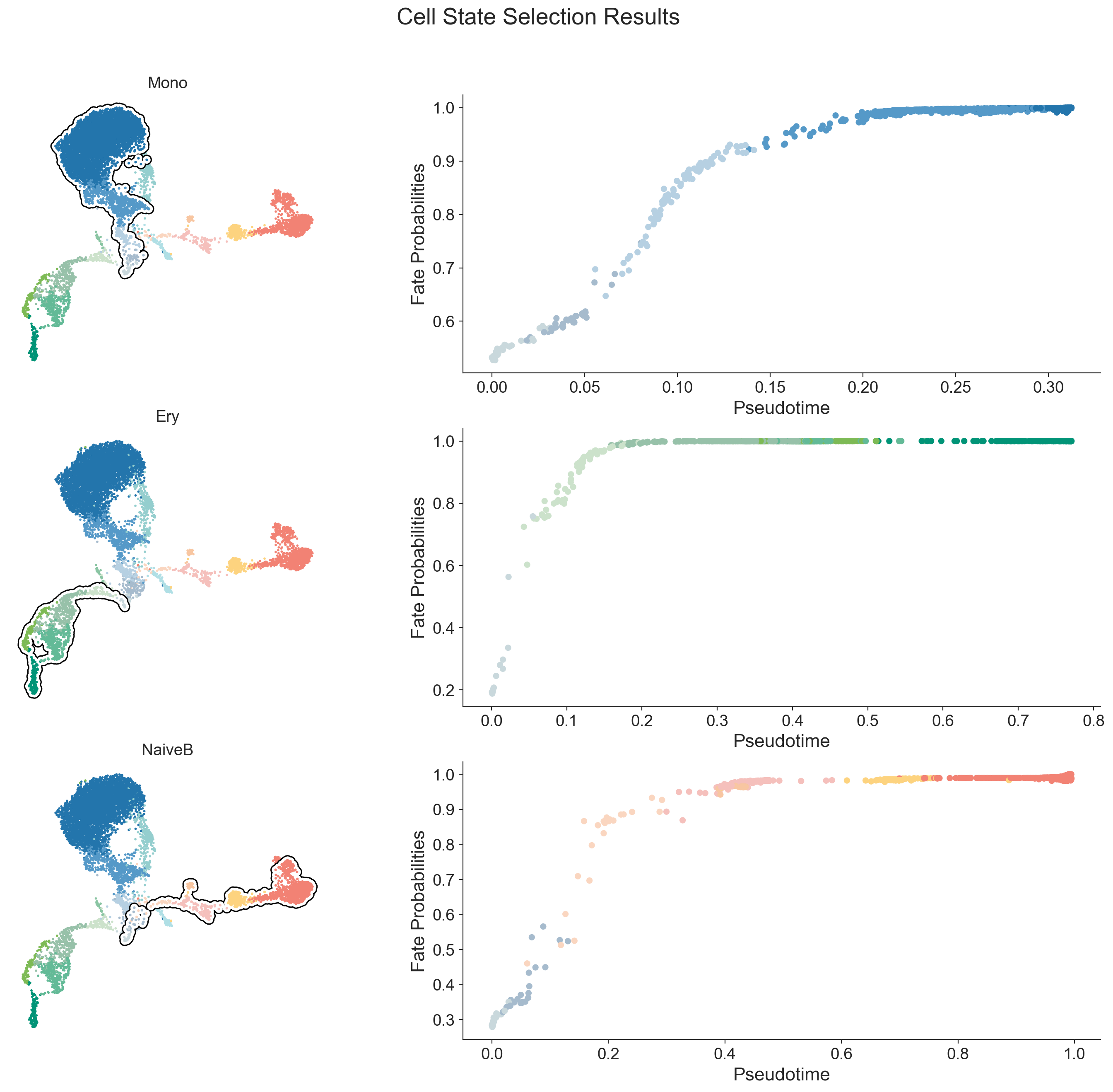
mdata.update()
Feature Association Test#
To identify genes that change significantly along pseudotime, we fit Generalized Additive Models (GAMs) on normalized counts using gaussian errors [FSKA23].
This approach is inspired by scFates, but other awesome methods for differential expression along pseudotime, such as PseudotimeDE [SL21] or Lamian [HJC+23], can also be applied.
mdata["RNA"].X = mdata["RNA"].layers["counts"].copy()
sc.pp.normalize_total(mdata["RNA"], target_sum=1e4)
sc.pp.log1p(mdata["RNA"])
mdata["RNA"].layers["log1p_norm"] = mdata["RNA"].X.copy()
We first run the association test on the log1p_norm layer. n_splines controls the GAM curve flexibility (see pyGAM documentation).
mdata = scm.tl.test_association(
    mdata, modal="RNA", layer="log1p_norm", A_cutoff=0.5, fdr_cutoff=1e-3, n_splines=5, n_jobs=10, recompute=True
)
INFO Running association test...
INFO Testing association between log1p_norm gene expression and palantir_pseudotime...
INFO     .varm['test_assoc_res'] --> added
         .uns['test_assoc'] --> added
          Feature Association Statistics
┏━━━━━━━━━━━━━━━━━━━━━━━━━━┳━━━━━━━━━━━━━━━━━━━━━━┓
┃                   Metric ┃ Value                ┃
┡━━━━━━━━━━━━━━━━━━━━━━━━━━╇━━━━━━━━━━━━━━━━━━━━━━┩
│              Total Genes │ 17,226               │
│               Thresholds │ FDR < 0.001, A > 0.5 │
│ Significant genes (n, %) │ 1,810 (10.51%)       │
└──────────────────────────┴──────────────────────┘
To efficiently test new thresholds, we simply call the function again. Since recompute defaults to False, this instantly updates the significant gene set using the new cutoffs without re-fitting models.
# Change cutoffs
mdata = scm.tl.test_association(
    mdata,
    A_cutoff=0.3,
    fdr_cutoff=1e-3,
)
INFO Using existing association test results.
          Feature Association Statistics
┏━━━━━━━━━━━━━━━━━━━━━━━━━━┳━━━━━━━━━━━━━━━━━━━━━━┓
┃                   Metric ┃ Value                ┃
┡━━━━━━━━━━━━━━━━━━━━━━━━━━╇━━━━━━━━━━━━━━━━━━━━━━┩
│              Total Genes │ 17,226               │
│               Thresholds │ FDR < 0.001, A > 0.3 │
│ Significant genes (n, %) │ 3,281 (19.05%)       │
└──────────────────────────┴──────────────────────┘
With the association test computed, let’s visualize the results for all genes, and let’s highlight a pre-defined set of key transcription factors using scm.pl.test_association().
key_TFs = ["PAX5", "EBF1", "TCF3", "IKZF1", "POU2F2", "FOXO1", "IRF4", "SOX4"]
scm.pl.test_association(mdata, A_cutoff=0.3, fdr_cutoff=1e-3, selected_genes=key_TFs)
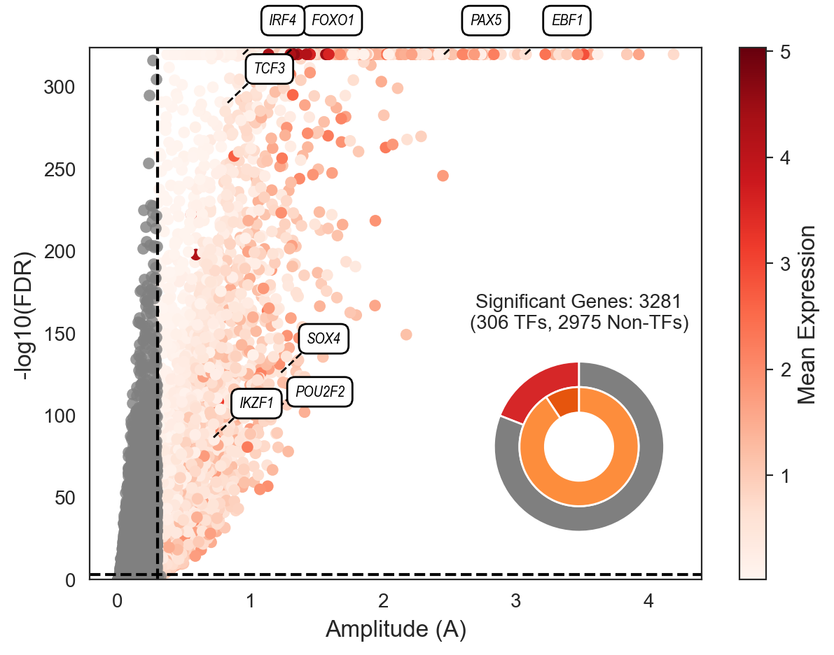
In the plot above, each dot represents a gene. The x-axis shows the amplitude (A) of its expression change along the trajectory, while the y-axis represents the statistical significance (-log10 FDR). Genes are colored by their mean expression.
We have highlighted several key_TFs known to be crucial for this B-cell differentiation process. The specific functions and literature references supporting the roles of these TFs are detailed in Supplementary Table 2 of the manuscript.
Visualize the Gene Expression Dynamics#
After identifying significant genes and classifying cells, we can visualize their expression dynamics along the inferred differentiation trajectory.
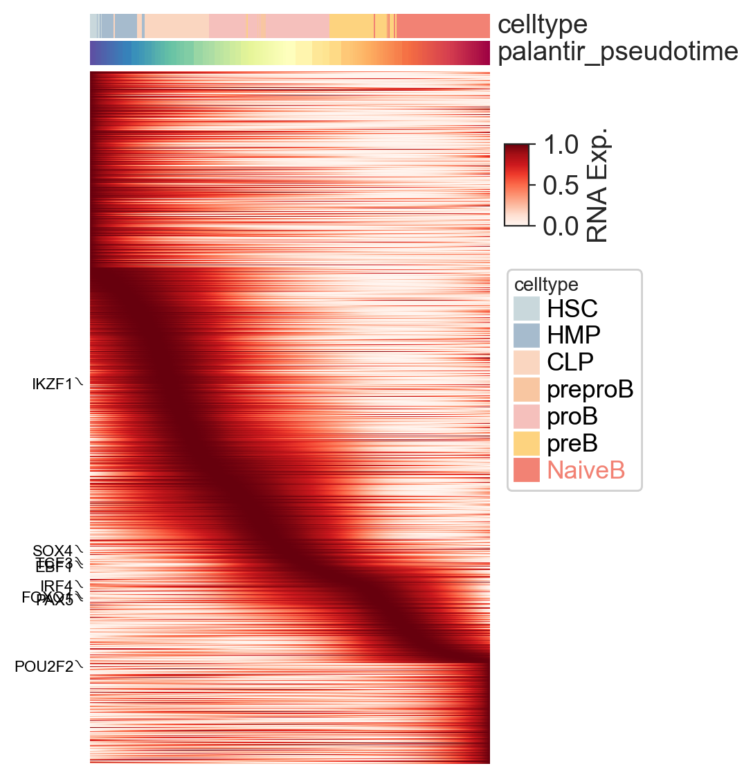
First, let’s plot a heatmap of all significant genes for the ‘NaiveB’ lineage, sorted by palantir_pseudotime. This gives a global overview of gene expression trends.
scm.pl.heatmap(
    mdata[mdata["RNA"].obsm["cell_state_masks"]["NaiveB"]],
    var_names=mdata["RNA"][:, mdata["RNA"].var["significant_genes"]].var_names,
    selected_genes=key_TFs,
    modal="RNA",
    layer="log1p_norm",
    sortby="palantir_pseudotime",
    col_annos=["celltype", "palantir_pseudotime"],
    smooth_method="gam",
    n_splines=5,
    cmap="Reds",
    label="RNA Exp.",
    figsize=(4, 6),
)
did not converge
To examine the behavior of individual genes, we can use scm.pl.trendplot. This plots the smoothed expression value of selected genes as a function of pseudotime.
We use the var_dict parameter to specify which features to plot: the dictionary keys (e.g., PAX5) set the names for the feature, while the values (e.g., [("RNA", "log1p_norm")]) define the modality and layer to pull the data from.
scm.pl.trendplot(
    mdata[mdata["RNA"].obsm["cell_state_masks"]["NaiveB"]],
    var_dict={"PAX5": [("RNA", "log1p_norm")], "EBF1": [("RNA", "log1p_norm")], "CD74": [("RNA", "log1p_norm")]},
    normalize=True,
    sortby="palantir_pseudotime",
    col_color=["celltype"],
    figsize=(6, 3),
    dpi=100,
    n_splines=5,
    show_tkey=False,
    show_stds=True,
)
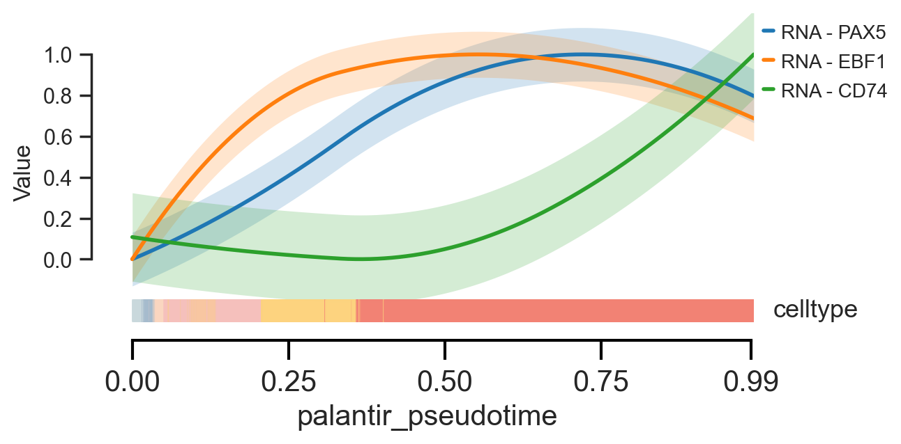
<Axes: xlabel='palantir_pseudotime', ylabel='Value'>
Several functions in scMagnify rely on data smoothing along pseudotime, offering multiple methods inspired by packages like cellRank and palantir.
The smooth_method parameter, available in the functions below, allows you to choose between:
'gam'(Generalized Additive Model)'convolve'(Moving average convolution)'polyfit'(Polynomial regression)
For full parameter details, please see the respective API documentation:
test_association()heatmap()trendplot()
For a deeper dive and usage examples, refer to the [Advanced Usage/Data Smoothing](./Advanced Usage/Data Smoothing.md) guide.
Save the data#
mdata.write(os.path.join(settings.data_dir, "mdata_tcelldep-bm_01.h5mu"))
Closing matters#
What’s next?#
In this tutorial, you learned how to preprocess scRNA-seq data to select cell states and their associated genes. For the next steps, we recommend the following:
Construct TF binding network with scATACseq and scRNAseq data
Refer to the {doc}API
to explore the available parameter values that can be used to customize these computations for your data.
If you encounter any bugs in the code, our if you have suggestions for new features, please open an issue. If you have a general question or something you would like to discuss with us, please post on the scverse discourse. You can also contact using chenxufeng2022@sinh.ac.cn.
Package versions#
import session_info

session_info.show()
Click to view session information
-----
anndata             0.9.2
cellrank            2.0.7
matplotlib          3.10.5
mudata              0.2.3
numba               0.61.2
numpy               1.26.4
pandas              2.3.1
scanpy              1.10.3
scmagnify           0.0.0
seaborn             0.13.2
session_info        v1.0.1
-----
Click to view modules imported as dependencies
MOODS                       NA
PIL                         11.3.0
PyComplexHeatmap            1.8.2
SEACells                    0.3.3
adjustText                  1.3.0
anyio                       NA
appdirs                     1.4.4
arrow                       1.3.0
asttokens                   NA
attr                        25.3.0
attrs                       25.3.0
babel                       2.17.0
backports                   NA
biothings_client            0.4.1
certifi                     2025.08.03
cffi                        1.17.1
charset_normalizer          3.4.2
click                       8.2.1
colorama                    0.4.6
comm                        0.2.3
cycler                      0.12.1
cython_runtime              NA
dateutil                    2.9.0.post0
debugpy                     1.8.17
decorator                   5.2.1
decoupler                   2.1.1
defusedxml                  0.7.1
deprecated                  1.2.18
dill                        0.4.0
diskcache                   5.6.3
docrep                      0.3.2
exceptiongroup              1.3.0
executing                   2.2.1
fastjsonschema              NA
filelock                    3.18.0
fqdn                        NA
genomepy                    0.16.1
grandalf                    NA
h5py                        3.14.0
httpx                       0.28.1
idna                        3.10
igraph                      0.11.9
ipykernel                   6.30.1
ipywidgets                  8.1.7
isoduration                 NA
jaraco                      NA
jax                         0.6.2
jaxlib                      0.6.2
jedi                        0.19.2
jinja2                      3.1.6
joblib                      1.5.1
json5                       0.12.0
jsonpointer                 3.0.0
jsonschema                  4.25.0
jsonschema_specifications   NA
jupyter_events              0.12.0
jupyter_server              2.16.0
jupyterlab_server           2.27.3
kiwisolver                  1.4.8
lark                        1.2.2
legacy_api_wrap             NA
legendkit                   0.3.6
llvmlite                    0.44.0
loguru                      0.7.3
markupsafe                  3.0.2
marsilea                    0.5.4
matplotlib_inline           0.1.7
ml_dtypes                   0.5.3
more_itertools              10.3.0
mpl_toolkits                NA
mpmath                      1.3.0
mygene                      3.2.2
mysql                       NA
natsort                     8.4.0
nbformat                    5.10.4
ncls                        NA
netgraph                    4.13.2
networkx                    3.4.2
norns                       NA
nvfuser                     NA
nvidia                      NA
opt_einsum                  3.4.0
overrides                   NA
packaging                   25.0
palantir                    1.4.1
palettable                  3.3.3
parso                       0.8.5
patsy                       1.0.1
petsc4py                    3.23.4
pkg_resources               NA
platformdirs                4.5.0
plotly                      6.3.0
pooch                       v1.8.2
progressbar                 4.5.0
prometheus_client           NA
prompt_toolkit              3.0.52
psutil                      7.1.0
pure_eval                   0.2.3
pyarrow                     20.0.0
pycparser                   2.22
pydev_ipython               NA
pydevconsole                NA
pydevd                      3.2.3
pydevd_file_utils           NA
pydevd_plugins              NA
pydevd_tracing              NA
pyfaidx                     0.8.1.4
pygam                       0.10.1
pygments                    2.19.2
pygpcca                     1.0.4
pyparsing                   3.2.3
pyranges                    0.1.4
pysam                       0.23.1
python_utils                NA
pythonjsonlogger            NA
pytz                        2025.2
referencing                 NA
requests                    2.32.4
rfc3339_validator           0.1.4
rfc3986_validator           0.1.1
rfc3987_syntax              NA
rich                        NA
rpack                       2.0.4
rpds                        NA
scipy                       1.15.3
scvelo                      0.3.3
send2trash                  NA
simplejson                  3.20.1
six                         1.17.0
sklearn                     1.5.2
slepc4py                    3.23.2
sniffio                     1.3.1
sorted_nearest              0.0.39
sphinxcontrib               NA
stack_data                  0.6.3
statsmodels                 0.14.5
swig_runtime_data4          NA
sympy                       1.14.0
tensorly                    0.9.0
texttable                   1.7.0
threadpoolctl               3.6.0
torch                       2.0.0+cu117
tornado                     6.5.2
tqdm                        4.67.1
traitlets                   5.14.3
typing_extensions           NA
uri_template                NA
urllib3                     2.5.0
vscode                      NA
wcwidth                     0.2.14
webcolors                   NA
websocket                   1.8.0
wrapt                       1.17.2
yaml                        6.0.2
zmq                         27.1.0
zoneinfo                    NA
-----
IPython             8.37.0
jupyter_client      8.6.3
jupyter_core        5.8.1
jupyterlab          4.4.5
-----
Python 3.10.18 | packaged by conda-forge | (main, Jun  4 2025, 14:45:41) [GCC 13.3.0]
Linux-5.14.0-503.31.1.el9_5.x86_64-x86_64-with-glibc2.34
-----
Session information updated at 2025-10-28 07:07