TF Binding Network Construction with scMagnify#
Preliminaries#
In this tutorial, you will learn how to:
Metacell/Pseudobulk Construction. Use
SEACells[PCD+23] to construct metacells from single-cell multiome data.cCREs Identification Identify significant peak–gene associations to get cCREs.
Motif Scan. Following the identification of cCREs, scMagnify scans the DNA sequences of candiate regions to identify transcription factor (TF)-binding motifs.
Note
This tutorial aims to assist users in preprocessing the scATACseq data for scMagnify analysis. For detailed instructions on the usage of SEACells, please refer to the official tutorial.
Import packages#
%load_ext autoreload
%autoreload 2
import warnings
from numba.core.errors import NumbaDeprecationWarning

warnings.simplefilter("ignore", category=NumbaDeprecationWarning)
warnings.simplefilter("ignore", FutureWarning)
warnings.simplefilter("ignore", UserWarning)
warnings.simplefilter("ignore", RuntimeWarning)
import os

import matplotlib.pyplot as plt
import scmagnify as scm
from scmagnify.settings import settings
scm.info()
 |
|
Configurations#
scm.settings.verbosity = 2
As in the previous tutorial, we first ensure the necessary built-in data is available. scMagnify will check the cache location; if the data is already present, it will not be downloaded again.
scm.datasets.fetch_scm_data()
INFO Data already processed and available at: /mnt/TrueNas/project/chenxufeng/Caches/scmagnify/scm_data
'/mnt/TrueNas/project/chenxufeng/Caches/scmagnify/scm_data'
%matplotlib inline

scm.settings.set_figure_params(
    dpi=100,
    facecolor="white",
    frameon=False,
)
# Load fonts from scm_data
scm.load_fonts(["Arial"])

plt.rcParams["font.family"] = "Arial"
plt.rcParams["grid.alpha"] = 0
# Setting a workspace
dirPjtHome = "/mnt/TrueNas/project/chenxufeng/Data/PMID36973557_NatBiotechnol2023_T-cell-depleted/"
workDir = os.path.join(dirPjtHome, "scmagnify_wd")
scm.set_workspace(workDir)
workspace: /mnt/TrueNas/project/chenxufeng/Data/PMID36973557_NatBiotechnol2023_T-cell-depleted/scmagnify_wd/
├── data
├── models
├── tmpfiles
└── figures
# Set up Reference Genome
scm.set_genome(version="hg38", genomes_dir="/home/chenxufeng/picb_cxf/Ref/human/hg38/")
                        Genome Information
┏━━━━━━━━━┳━━━━━━━━━━┳━━━━━━━━━━━━━━━━━━━━━━━━━━━━━━━━━━━━━━━━━━━┓
┃ Version ┃ Provider ┃ Directory                                 ┃
┡━━━━━━━━━╇━━━━━━━━━━╇━━━━━━━━━━━━━━━━━━━━━━━━━━━━━━━━━━━━━━━━━━━┩
│ hg38    │ UCSC     │ /home/chenxufeng/picb_cxf/Ref/human/hg38/ │
└─────────┴──────────┴───────────────────────────────────────────┘
Load the data#
mdata = scm.read(os.path.join(settings.data_dir, "mdata_tcelldep-bm_01.h5mu"))
mdata
MuData object with n_obs × n_vars = 8627 × 233703
  2 modalities
    ATAC:	8627 x 216477
      obs:	'Sample', 'TSSEnrichment', 'ReadsInTSS', 'ReadsInPromoter', 'ReadsInBlacklist', 'PromoterRatio', 'PassQC', 'NucleosomeRatio', 'nMultiFrags', 'nMonoFrags', 'nFrags', 'nDiFrags', 'BlacklistRatio', 'Clusters', 'ReadsInPeaks', 'FRIP', 'leiden', 'phenograph', 'celltype', 'SEACell', 'sample'
      var:	'seqnames', 'start', 'end', 'width', 'strand', 'score', 'replicateScoreQuantile', 'groupScoreQuantile', 'Reproducibility', 'GroupReplicate', 'nearestGene', 'distToGeneStart', 'peakType', 'distToTSS', 'nearestTSS', 'GC', 'idx', 'N', 'Bcells_primed', 'Bcells_lineage_specific'
      uns:	'FIMOColumns', 'GeneScoresColumns', 'InSilicoChipColumns', 'celltype_colors', 'celltype_combined_colors', 'leiden', 'leiden_colors', 'neighbors', 'phenograph_colors', 'tab20', 'umap'
      obsm:	'DM_EigenVectors', 'GeneScores', 'X_svd', 'X_umap'
      varm:	'FIMO', 'InSilicoChip', 'InSilicoChip_Corrs', 'OpenPeaks'
      layers:	'counts', 'tf_idf'
      obsp:	'ImputeWeights', 'connectivities', 'distances'
    RNA:	8627 x 17226
      obs:	'sample', 'celltype', 'palantir_pseudotime', 'macrostates_fwd', 'clusters_gradients', 'term_states_fwd', 'term_states_fwd_probs', 'init_states_fwd', 'init_states_fwd_probs'
      var:	'highly_variable', 'means', 'dispersions', 'dispersions_norm'
      uns:	'T_fwd_params', 'celltype_colors', 'clusters_gradients_colors', 'coarse_fwd', 'custom_branch_mask_columns', 'dea_celltype', 'dendrogram_celltype', 'eigendecomposition_fwd', 'hvg', 'init_states_fwd_colors', 'lineage_colors', 'log1p', 'macrostates_fwd_colors', 'neighbors', 'pca', 'sample_colors', 'schur_matrix_fwd', 'term_states_fwd_colors', 'umap'
      obsm:	'T_fwd_umap', 'X_FDL', 'X_fate_simplex_fwd', 'X_pca', 'X_umap', 'branch_masks', 'cell_state_masks', 'cellrank_branch_masks', 'cellrank_fate_probabilities', 'cellrank_masks', 'init_states_fwd_memberships', 'lineages_fwd', 'macrostates_fwd_memberships', 'palantir_branch_probs', 'palantir_fate_probabilities', 'palantir_lineage_cells', 'schur_vectors_fwd'
      varm:	'PCs', 'geneXTF'
      layers:	'MAGIC_imputed_data', 'counts'
      obsp:	'connectivities', 'distances', 'knn'
Metacell/Pseudobulk construction#
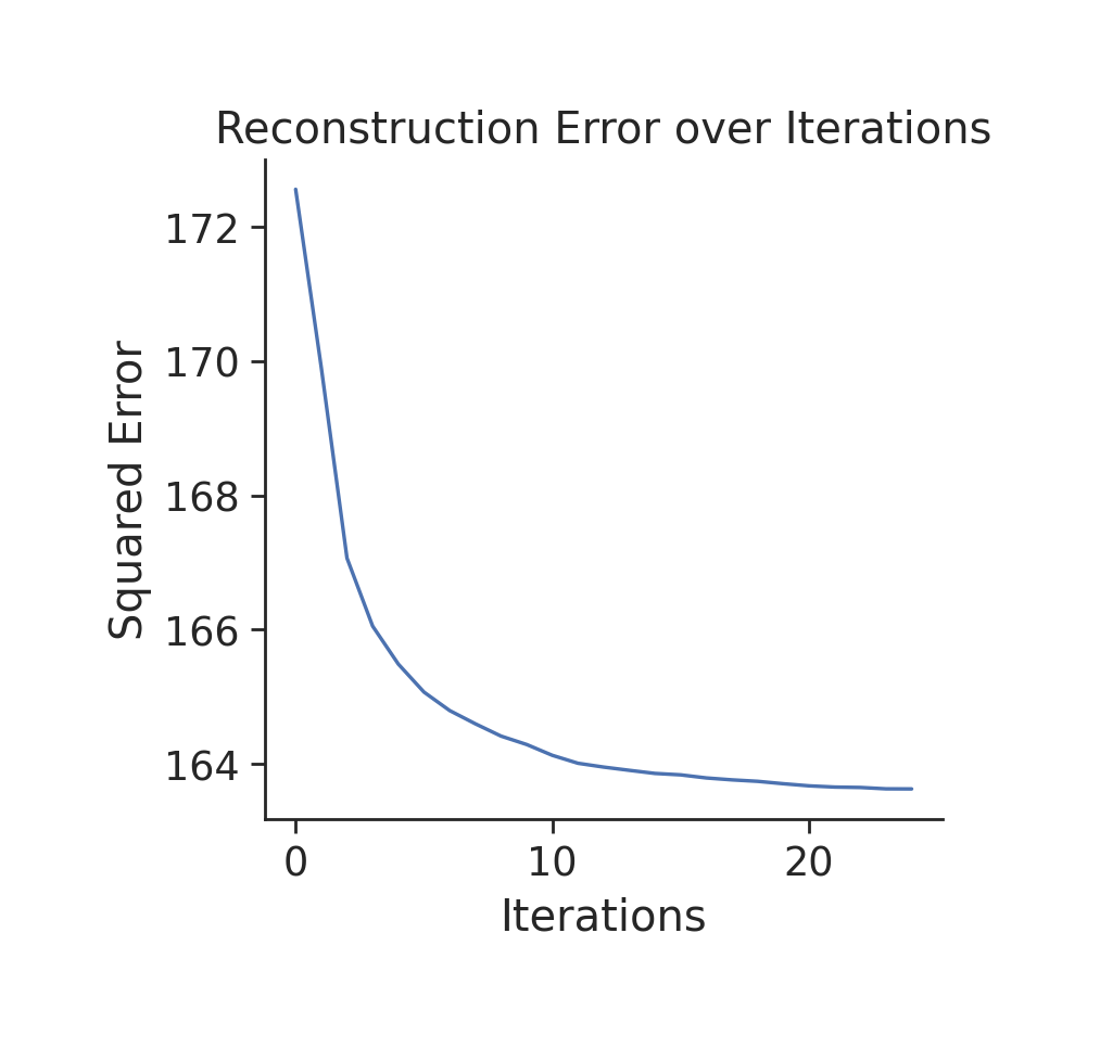
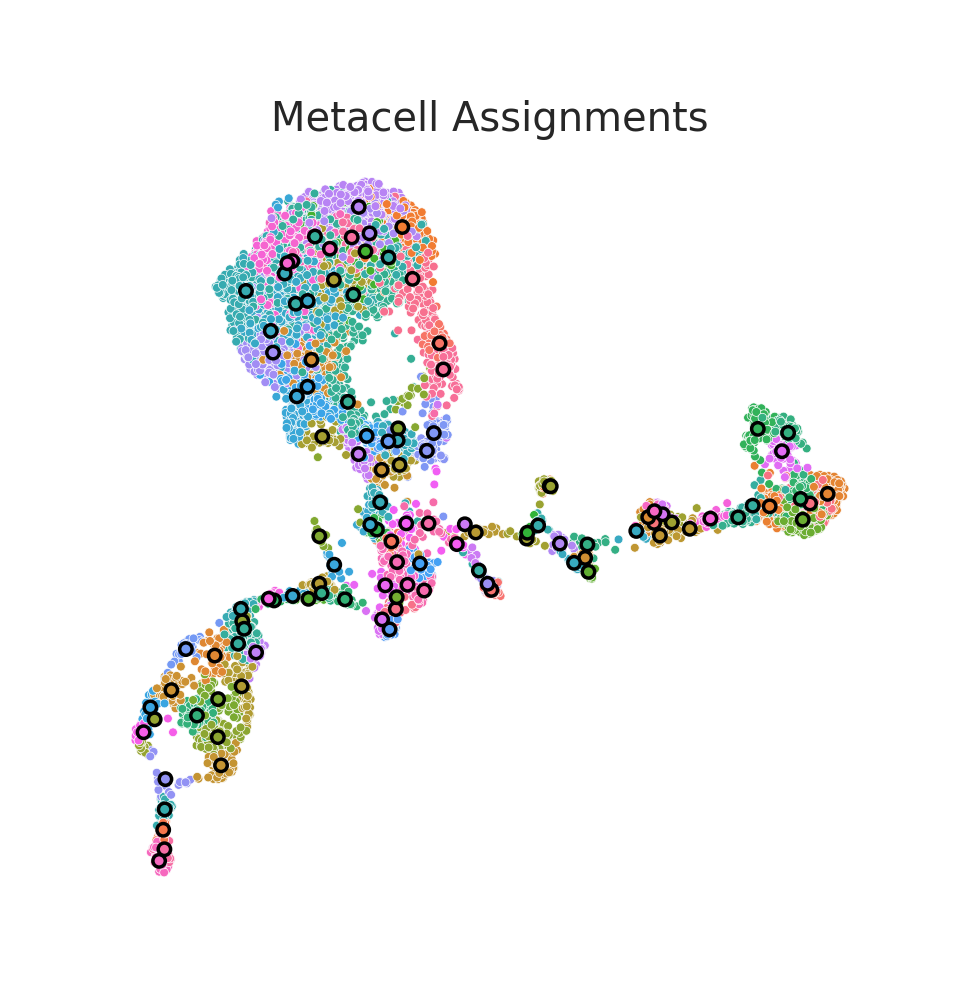
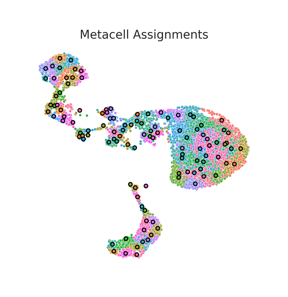
scMagnify utilizes SEACells [PCD+23] to construct metacells, which represent robust cellular states by aggregating data from groups of similar single cells.
We use the scm.tl.build_metacells_SEACells wrapper function for this process. This function builds the metacells based on a specified dimensionality reduction (DR) result—in this case, the X_pca from the RNA modality (as set by rna_dr_key).
Once the metacells are defined, the function aggregates the raw counts from both the RNA and ATAC layers (rna_layer, atac_layer). It also summarizes other important metadata from adata.obs, such as celltype (defined by groupby) and palantir_pseudotime (defined by t_key), into the new meta_mdata object.
meta_mdata = scm.tl.build_metacells_SEACells(
    mdata,
    rna_key="RNA",
    atac_key="ATAC",
    rna_dr_key="X_pca",
    atac_dr_key="X_svd",
    rna_layer="counts",
    atac_layer="counts",
    groupby="celltype",
    mask_key="cell_state_masks",
    embed_key="X_umap",
    t_key="palantir_pseudotime",
    use_gpu=True,
)
INFO Using layer: counts
WARNING: adata.X seems to be already log-transformed.
Welcome to SEACells!
Computing kNN graph using scanpy NN ...
Computing radius for adaptive bandwidth kernel...
Making graph symmetric...
Parameter graph_construction = union being used to build KNN graph...
Computing RBF kernel...
Building similarity LIL matrix...
Constructing CSR matrix...
Building kernel on X_pca
Computing diffusion components from X_pca for waypoint initialization ...
Determing nearest neighbor graph...
Done.
Sampling waypoints ...
Done.
Selecting 100 cells from waypoint initialization.
Initializing residual matrix using greedy column selection
Initializing f and g...
Selecting 15 cells from greedy initialization.
Randomly initialized A matrix.
Setting convergence threshold at 0.00173
Starting iteration 1.
Completed iteration 1.
Starting iteration 10.
Completed iteration 10.
Starting iteration 20.
Completed iteration 20.
Converged after 24 iterations.
Welcome to SEACells!
Computing kNN graph using scanpy NN ...
Computing radius for adaptive bandwidth kernel...
Making graph symmetric...
Parameter graph_construction = union being used to build KNN graph...
Computing RBF kernel...
Building similarity LIL matrix...
Constructing CSR matrix...
Building kernel on X_svd
Computing diffusion components from X_svd for waypoint initialization ...
Determing nearest neighbor graph...
Done.
Sampling waypoints ...
Done.
Selecting 104 cells from waypoint initialization.
Initializing residual matrix using greedy column selection
Initializing f and g...
Selecting 11 cells from greedy initialization.
Randomly initialized A matrix.
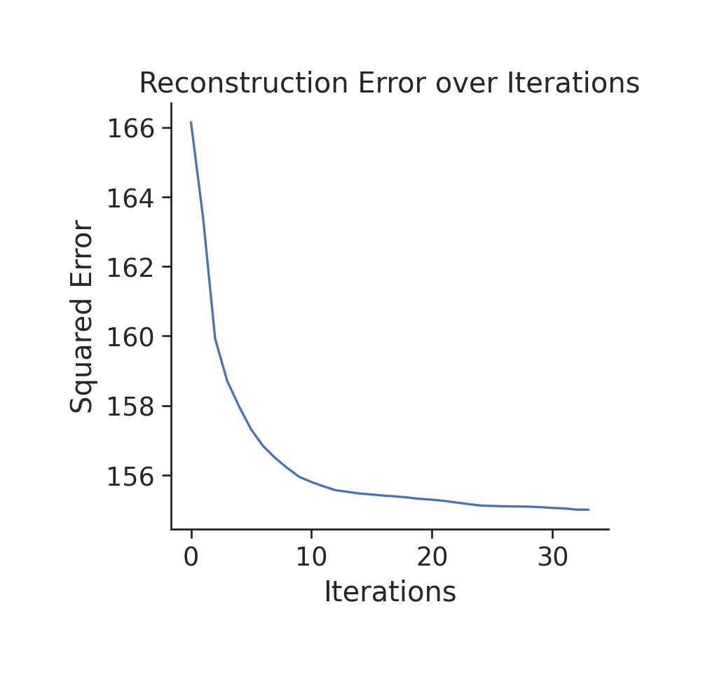
Setting convergence threshold at 0.00166
Starting iteration 1.
Completed iteration 1.
Starting iteration 10.
Completed iteration 10.
Starting iteration 20.
Completed iteration 20.
Starting iteration 30.
Completed iteration 30.
Converged after 33 iterations.
Generating Metacell matrices...
ATAC
RNA
INFO Running SEACells model for RNA data...
INFO Running SEACells model for ATAC data...
INFO Assigning celltype to metacells...
INFO Assigning cell_state_masks to metacells...
Conduct lineage-specifc scATACseq analysis#
We will now demonstrate the lineage-specific analysis workflow. For this tutorial, we will select the ‘NaiveB’ lineage as our target of interest.
cell_state = "NaiveB"
Peak-gene correlation test#
A key step in building a GRN is to link distal regulatory elements (peaks, or cCREs) to their potential target genes. Here, we identify peak-gene pairs by correlating peak accessibility and gene expression across metacells within our selected lineage.
First, we filter both the single-cell (mdata) and metacell (meta_mdata) objects to include only the ‘NaiveB’ cells.
mdata_fil = mdata[mdata["RNA"].obsm["cell_state_masks"][cell_state]].copy()
meta_mdata_fil = meta_mdata[meta_mdata.obsm["cell_state_masks"][cell_state]].copy()
Next, we run scm.tl.connect_peaks_genes. This function computes a Pearson correlation between gene expression and peak accessibility using the aggregated meta_mdata_fil object.
The current implementation is inspired by the SEACells tfactivity.py module (see source code).
Note
We are actively working on integrating additional peak-to-gene linkage methods. scMagnify also supports importing pre-computed peak-gene associations derived from other algorithms.
mdata_fil = scm.tl.connect_peaks_genes(mdata_fil, meta_mdata_fil, cor_cutoff=0.1, pval_cutoff=0.1, n_jobs=20)
INFO Loading transcripts from GTF file...
INFO Calculating peak-gene correlations...
/picb/lihonglab/chenxufeng/miniconda3/envs/scm_test/lib/python3.10/site-packages/joblib/externals/loky/process_exec
utor.py:782: UserWarning: A worker stopped while some jobs were given to the executor. This can be caused by a too
short worker timeout or by a memory leak.
  warnings.warn(
/picb/lihonglab/chenxufeng/miniconda3/envs/scm_test/lib/python3.10/site-packages/joblib/externals/loky/process_exec
utor.py:782: UserWarning: A worker stopped while some jobs were given to the executor. This can be caused by a too
short worker timeout or by a memory leak.
  warnings.warn(
/picb/lihonglab/chenxufeng/miniconda3/envs/scm_test/lib/python3.10/site-packages/joblib/externals/loky/process_exec
utor.py:782: UserWarning: A worker stopped while some jobs were given to the executor. This can be caused by a too
short worker timeout or by a memory leak.
  warnings.warn(
/picb/lihonglab/chenxufeng/miniconda3/envs/scm_test/lib/python3.10/site-packages/joblib/externals/loky/process_exec
utor.py:782: UserWarning: A worker stopped while some jobs were given to the executor. This can be caused by a too
short worker timeout or by a memory leak.
  warnings.warn(
/picb/lihonglab/chenxufeng/miniconda3/envs/scm_test/lib/python3.10/site-packages/joblib/externals/loky/process_exec
utor.py:782: UserWarning: A worker stopped while some jobs were given to the executor. This can be caused by a too
short worker timeout or by a memory leak.
  warnings.warn(
/picb/lihonglab/chenxufeng/miniconda3/envs/scm_test/lib/python3.10/site-packages/joblib/externals/loky/process_exec
utor.py:782: UserWarning: A worker stopped while some jobs were given to the executor. This can be caused by a too
short worker timeout or by a memory leak.
  warnings.warn(
/picb/lihonglab/chenxufeng/miniconda3/envs/scm_test/lib/python3.10/site-packages/joblib/externals/loky/process_exec
utor.py:782: UserWarning: A worker stopped while some jobs were given to the executor. This can be caused by a too
short worker timeout or by a memory leak.
  warnings.warn(
/picb/lihonglab/chenxufeng/miniconda3/envs/scm_test/lib/python3.10/site-packages/joblib/externals/loky/process_exec
utor.py:782: UserWarning: A worker stopped while some jobs were given to the executor. This can be caused by a too
short worker timeout or by a memory leak.
  warnings.warn(
/picb/lihonglab/chenxufeng/miniconda3/envs/scm_test/lib/python3.10/site-packages/joblib/externals/loky/process_exec
utor.py:782: UserWarning: A worker stopped while some jobs were given to the executor. This can be caused by a too
short worker timeout or by a memory leak.
  warnings.warn(
/picb/lihonglab/chenxufeng/miniconda3/envs/scm_test/lib/python3.10/site-packages/joblib/externals/loky/process_exec
utor.py:782: UserWarning: A worker stopped while some jobs were given to the executor. This can be caused by a too
short worker timeout or by a memory leak.
  warnings.warn(
/picb/lihonglab/chenxufeng/miniconda3/envs/scm_test/lib/python3.10/site-packages/joblib/externals/loky/process_exec
utor.py:782: UserWarning: A worker stopped while some jobs were given to the executor. This can be caused by a too
short worker timeout or by a memory leak.
  warnings.warn(
                  Peak-Gene Correlations Summary
┏━━━━━━━━━━━━━━━━━━━━━━━━━━━━━┳━━━━━━━━━━━━━━━━━━━━━━━━━━━━━━━━━━┓
┃                      Metric ┃ Value                            ┃
┡━━━━━━━━━━━━━━━━━━━━━━━━━━━━━╇━━━━━━━━━━━━━━━━━━━━━━━━━━━━━━━━━━┩
│             Number of genes │ 3281                             │
│             Number of peaks │ 216477                           │
│                     Cutoffs │ Correlation > 0.1, P-value < 0.1 │
│ Number of significant peaks │ 24441                            │
│ Number of significant genes │ 3173                             │
└─────────────────────────────┴──────────────────────────────────┘
Motif Scanning#
After identifying the peak-gene links, the next step is to determine which TFs bind to these peaks (cCREs). We use MotifScanner to scan the DNA sequence of each peak for known TF binding motifs.
This tool is built upon the MOODS library [KMartinmakiP+] for efficient Position Weight Matrix (PWM) matching. For detailed explanations of scanning parameters and the underlying principles, please refer to the MOODS documentation.
First, we import and initialize the scanner. While the default database is the HOCOMOCOv11_CORE collection
from scmagnify.tools import MotifScanner
You can list all available built-in databases at any time.
Finally, we call the scanner.match() method on our filtered mdata object. This scans all peaks defined in mdata_fil.var and stores the resulting motif scanning results in mdata_fil.uns[‘motif_scan’].
scanner = MotifScanner(motif_db="HOCOMOCOv11_HUMAN")
INFO     Importing motifs from
         '/home/chenxufeng/WorkSpace/Git-repos/scMagnify/src/scmagnify/data/motifs/HOCOMOCOv11_HUMAN.pfm' in PFM
         format...
INFO     Successfully imported 401 new motifs.
         Total motifs in scanner: 401.
scanner.show_motif_databases()
               Available Motif Databases
┏━━━━━━━━━━━━━━━━━━━┳━━━━━━━━━━━━━━━━━━┳━━━━━━━━━━━━━━━┓
┃ Motif Database    ┃ Number of Motifs ┃ Number of TFs ┃
┡━━━━━━━━━━━━━━━━━━━╇━━━━━━━━━━━━━━━━━━╇━━━━━━━━━━━━━━━┩
│ CIS-BP            │            10033 │     5600      │
│ CIS-BP_FigR_HUMAN │             1141 │     1141      │
│ CIS-BP_FigR_MOUSE │              890 │      890      │
│ HOCOMOCOv11_HUMAN │              401 │      401      │
│ HOCOMOCOv11_MOUSE │              356 │      356      │
│ HOCOMOCOv13_HUMAN │             1611 │     1109      │
│ HOCOMOCOv13_MOUSE │             1253 │      811      │
│ HOMER             │              436 │      428      │
└───────────────────┴──────────────────┴───────────────┘
mdata_fil = scanner.match(mdata_fil)
        Motif Scan Summary
┏━━━━━━━━━━━━━━━━━━━━━━━━━┳━━━━━━━┓
┃                  Metric ┃ Value ┃
┡━━━━━━━━━━━━━━━━━━━━━━━━━╇━━━━━━━┩
│   Number of motifs used │ 401   │
│ Number of peaks scanned │ 24441 │
│      Final score cutoff │ > 0   │
└─────────────────────────┴───────┘
Save the data#
mdata_fil.write(os.path.join(settings.data_dir, "mdata_tcelldep-bm_02_NaiveB.h5mu"))
meta_mdata_fil.write(os.path.join(settings.data_dir, "meta_mdata_tcelldep-bm_02_NaiveB.h5ad"))
Closing matters#
What’s next?#
In this tutorial, you learned how to build metacells with SEACells, perform peak-gene correlation, and use MotifScanner to construct a high-confidence TF binding network.
You now have both required inputs:
Dynamic gene expression (from Tutorial 1)
A TF binding network (from this tutorial)
For the next steps, we recommend the following:
Proceed to the next tutorial to Infer the Multi-scale Gene Regulatory Network. This step combines both inputs using the
scm.MAGNImodel to infer the GRN and calculate TF activities.Refer to the API to explore the available parameter values that can be used to customize these computations for your data.
If you encounter any bugs or have suggestions for new features, please open an issue. For general questions, please post on the scverse discourse or contact us at chenxufeng2022@sinh.ac.cn.
Package versions#
import session_info

session_info.show()