Multi-scale Gene Regulation Inference and Analysis with scMagnify#
Preliminaries#
In this tutorial, you will learn how to:
Multi-scale Gene Regulation Inference. scMagnify builds upon nonlinear multivariable Granger causal inference, implemented through an interpretable multi-scale neural network.
Key Regulators Characterization. Identify critical regulators by first performing Regulatory Activity Inference to estimate TF activities, and then using Network Score Calculation (based on graph theory) to rank their importance in the network.
See our manuscript for more details.
Input#
scMagnify uses two types of input data during the regulation inference.
Input data 1: scRNA-seq data. Please look at the previous section to learn about the scRNA-seq data preprocessing and cell state dynamics analysis.
Input data 2: TF Binding Network. The TF binding network represents the TF-TG connections. The data structure is a binary 2D matrix or linklist. You can construct the binary network following our workflow, or alternatively, provide a custom one.
GRNMuData#
The GRNMuData class extends the MuData class to incorporate Gene Regulatory Networks (GRNs) and associated analysis results. Additionally, it provides a set of functions for network pruning and object conversion. Subsequent analyses will be based on this object.
For a detailed explanation of the model architecture and the theory behind our Multi-scale Neural Granger Causality (MSNGC) framework, please refer to the **[About the scMagnify](./About the MSNGC.md)** section.
:::
Import packages#
%load_ext autoreload
%autoreload 2
import warnings
from numba.core.errors import NumbaDeprecationWarning

warnings.simplefilter("ignore", category=NumbaDeprecationWarning)
warnings.simplefilter("ignore", FutureWarning)
warnings.simplefilter("ignore", UserWarning)
warnings.simplefilter("ignore", RuntimeWarning)
import os

import matplotlib.pyplot as plt
import scanpy as sc
import scmagnify as scm
from scmagnify.settings import settings
scm.info()
 |
|
Configurations#
scm.settings.verbosity = 2
%matplotlib inline

scm.settings.set_figure_params(
    dpi=100,
    facecolor="white",
    frameon=False,
)

scm.load_fonts(["Arial"])

plt.rcParams["font.family"] = "Arial"
plt.rcParams["grid.alpha"] = 0
# Setting a workspace
dirPjtHome = "/mnt/TrueNas/project/chenxufeng/Data/PMID36973557_NatBiotechnol2023_T-cell-depleted/"
workDir = os.path.join(dirPjtHome, "scmagnify_wd")
scm.set_workspace(workDir)
workspace: /mnt/TrueNas/project/chenxufeng/Data/PMID36973557_NatBiotechnol2023_T-cell-depleted/scmagnify_wd/
├── data
├── models
├── tmpfiles
└── figures
# Set up Reference Genome
scm.set_genome(version="hg38", genomes_dir="/home/chenxufeng/picb_cxf/Ref/human/hg38/")
                        Genome Information
┏━━━━━━━━━┳━━━━━━━━━━┳━━━━━━━━━━━━━━━━━━━━━━━━━━━━━━━━━━━━━━━━━━━┓
┃ Version ┃ Provider ┃ Directory                                 ┃
┡━━━━━━━━━╇━━━━━━━━━━╇━━━━━━━━━━━━━━━━━━━━━━━━━━━━━━━━━━━━━━━━━━━┩
│ hg38    │ UCSC     │ /home/chenxufeng/picb_cxf/Ref/human/hg38/ │
└─────────┴──────────┴───────────────────────────────────────────┘
Load the data#
mdata = scm.read(os.path.join(scm.settings.data_dir, "t-cell-depleted-bm_NaiveB_H11CORE_02.h5mu"))
mdata
MuData object with n_obs × n_vars = 1374 × 233703
  uns:	'motif_scan', 'peak_gene_corrs'
  obsm:	'cell_state_masks'
  2 modalities
    ATAC:	1374 x 216477
      obs:	'sample', 'celltype', 'TSSEnrichment', 'NucleosomeRatio', 'nFrags', 'BlacklistRatio', 'SEACell'
      var:	'seqnames', 'start', 'end', 'strand', 'GC', 'Bcells_primed', 'Bcells_lineage_specific'
      uns:	'celltype_colors', 'neighbors', 'peak_seq', 'sample_colors', 'umap'
      obsm:	'DM_EigenVectors', 'GeneScores', 'X_svd', 'X_umap'
      layers:	'counts'
      obsp:	'connectivities', 'distances'
    RNA:	1374 x 17226
      obs:	'sample', 'celltype', 'palantir_pseudotime', 'macrostates_fwd', 'term_states_fwd', 'term_states_fwd_probs', 'clusters_gradients', 'init_states_fwd', 'init_states_fwd_probs', 'n_counts', 'SEACell'
      var:	'highly_variable', 'significant_genes', 'means', 'dispersions', 'dispersions_norm'
      uns:	'T_fwd_params', 'celltype_colors', 'clusters_gradients_colors', 'coarse_fwd', 'eigendecomposition_fwd', 'hvg', 'init_states_fwd_colors', 'log1p', 'macrostates_fwd_colors', 'neighbors', 'sample_colors', 'schur_matrix_fwd', 'term_states_fwd_colors', 'test_assoc', 'umap'
      obsm:	'T_fwd_umap', 'X_FDL', 'X_fate_simplex_fwd', 'X_pca', 'X_umap', 'cell_state_masks', 'cellrank_fate_probabilities', 'init_states_fwd_memberships', 'lineages_fwd', 'macrostates_fwd_memberships', 'schur_vectors_fwd'
      varm:	'test_assoc_res'
      layers:	'MAGIC_imputed_data', 'counts', 'log1p_norm'
      obsp:	'connectivities', 'distances', 'knn'
Train the model#
After preparing the scRNA-seq data and constructing the TF binding network, we are ready to infer the multi-scale GRN.
The first step is to initialize the scm.MAGNI model. This initialization call handles more than just setting parameters; it also performs all necessary data preprocessing based on the mdata object and the previously defined TF binding network:
It maps the motif-based TF binding network to the genes and TFs present in the RNA expression data.
It builds the chromatin constraint statistics.
It normalizes the expression data from the specified
layer.It constructs the internal data structures (like the DAG and S matrix) required by the MSNGC model.
It sets up the model architecture (e.g.,
hiddenlayers) and moves it to the specifieddevice.
magni = scm.MAGNI(
    mdata, max_iter=1000, patience=10, layer="log1p_norm", hidden=[50], lag=5, batch_size=32, seed=42, device="cuda:1"
)
   Chromatin Constraint Statistics
┏━━━━━━━━━━━━━━━━━━━━━━━━━━━┳━━━━━━━┓
┃ Metric                    ┃ Value ┃
┡━━━━━━━━━━━━━━━━━━━━━━━━━━━╇━━━━━━━┩
│ n_cells                   │  1374 │
│ n_genes                   │ 17226 │
│ n_regulators_in_basal_GRN │   403 │
│ n_targets_in_basal_GRN    │  2927 │
│ n_regulators_in_both      │   105 │
│ n_targets_in_both         │  2928 │
└───────────────────────────┴───────┘
INFO Normalizing data: 0 mean, 1 SD
INFO Constructing DAG...
INFO Constructing S matrix...
INFO Calculating diffusion lags...
INFO     MSNGC(
           (coeff_nets): ModuleList(
             (0-4): 5 x Sequential(
               (0): Sequential(
                 (0): Linear(in_features=105, out_features=50, bias=True)
                 (1): ReLU()
               )
               (1): Linear(in_features=50, out_features=307440, bias=True)
             )
           )
           (attention): Embedding(1, 5)
         )
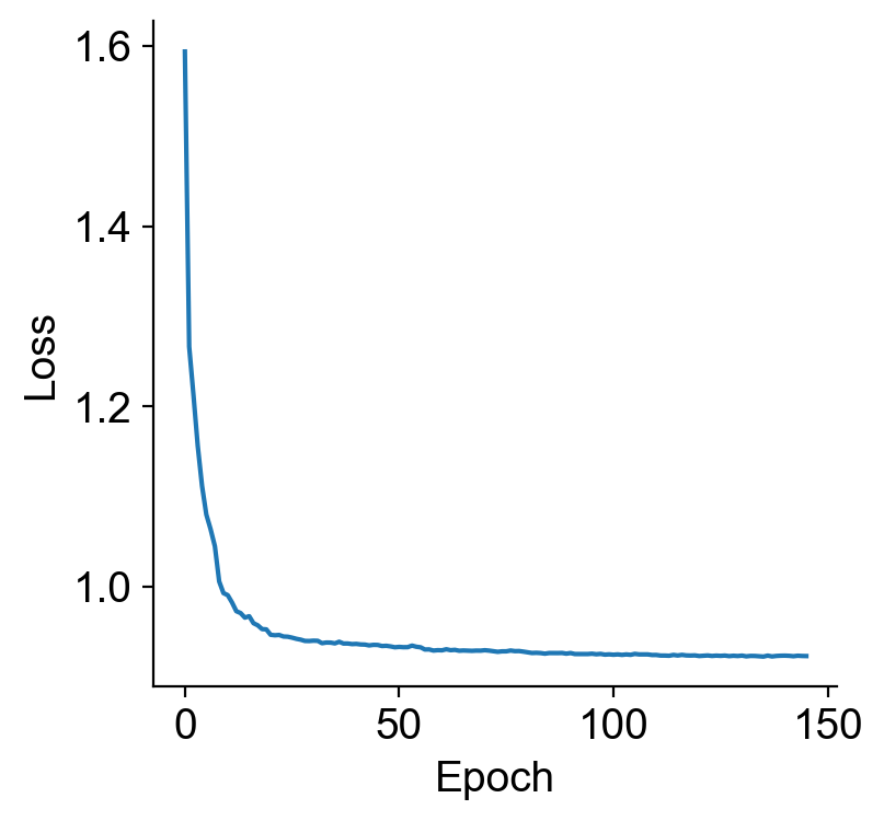
model = magni.train()
Epoch 00056: reducing learning rate of group 0 to 5.0000e-04.
Epoch 00080: reducing learning rate of group 0 to 2.5000e-04.
Epoch 00091: reducing learning rate of group 0 to 1.2500e-04.
Epoch 00109: reducing learning rate of group 0 to 6.2500e-05.
Epoch 00120: reducing learning rate of group 0 to 3.1250e-05.
Epoch 00127: reducing learning rate of group 0 to 1.5625e-05.
Epoch 00142: reducing learning rate of group 0 to 7.8125e-06.
INFO Early stopping at epoch 145
plt.plot(model.history["train_loss"])
plt.xlabel("Epoch")
plt.ylabel("Loss")
plt.show()
magni.save(os.path.join(settings.models_dir, "t-cell-depleted-bm_NaiveB_02_MAGNI_model.pth"))
INFO     Saving model state to
         /mnt/TrueNas/project/chenxufeng/Data/PMID36973557_NatBiotechnol2023_T-cell-depleted/scmagnify_wd/models/t-
         cell-depleted-bm_NaiveB_02_MAGNI_model.pth...
INFO Model saved successfully.
Regulation Inference#
Once the model is initialized and data is preprocessed, we call the magni.regulation_inference() method to run the model and infer the network.
This single function executes the complete inference and post-processing pipeline:
It use the trained MSNGC model to find causal relationships.
It estimates time lags and formulates the initial network edges.
It computes the regulatory activity for each TF.
It filters the network edges based on coefficient scores (e.g., using a quantile cutoff) to prune weak or noisy connections.
Finally, it bundles all results—including the filtered network, TF activities, and attention weights—into a new
GRNMuDataobject for downstream analysis.
gdata = magni.regulation_inference()
INFO Starting regulation inference...
INFO Computing CV of the coefficients with 0.2...
INFO Estimating time lags...
INFO Formulating network edges...
INFO Computing TF activity...
INFO Creating GRNMuData object...
INFO Filtering network by quantile with params 0.9...
                                 Network Filtered Statistics
┏━━━━━━━━━━━━━━━━━━━━━━┳━━━━━━━━━━━━━━━━━━━━━━┳━━━━━━━━━━━━━━━━━━━━━━┳━━━━━━━━━━━━━━━━━━━━━━┓
┃ Method(Param)        ┃ Attribute            ┃ Binarize             ┃ Filtered/Raw(Percen… ┃
┡━━━━━━━━━━━━━━━━━━━━━━╇━━━━━━━━━━━━━━━━━━━━━━╇━━━━━━━━━━━━━━━━━━━━━━╇━━━━━━━━━━━━━━━━━━━━━━┩
│ quantile(0.9)        │ score                │ True                 │ 7922/79219 (0.10)    │
└──────────────────────┴──────────────────────┴──────────────────────┴──────────────────────┘
INFO Saving attention weights...
gdata
Gene Regulatory Network (GRN) with 79219 edges.
MuData object with n_obs × n_vars = 1374 × 233808
  uns:	'motif_scan', 'peak_gene_corrs', 'network', 'filtered_network', 'attention_weights'
  3 modalities
    ATAC:	1374 x 216477
      obs:	'sample', 'celltype', 'TSSEnrichment', 'NucleosomeRatio', 'nFrags', 'BlacklistRatio', 'SEACell'
      var:	'seqnames', 'start', 'end', 'strand', 'GC', 'Bcells_primed', 'Bcells_lineage_specific'
      uns:	'celltype_colors', 'neighbors', 'peak_seq', 'sample_colors', 'umap'
      obsm:	'DM_EigenVectors', 'GeneScores', 'X_svd', 'X_umap'
      layers:	'counts'
      obsp:	'connectivities', 'distances'
    RNA:	1374 x 17226
      obs:	'sample', 'celltype', 'palantir_pseudotime', 'macrostates_fwd', 'term_states_fwd', 'term_states_fwd_probs', 'clusters_gradients', 'init_states_fwd', 'init_states_fwd_probs', 'n_counts', 'SEACell'
      var:	'highly_variable', 'significant_genes', 'means', 'dispersions', 'dispersions_norm'
      uns:	'T_fwd_params', 'celltype_colors', 'clusters_gradients_colors', 'coarse_fwd', 'eigendecomposition_fwd', 'hvg', 'init_states_fwd_colors', 'log1p', 'macrostates_fwd_colors', 'neighbors', 'sample_colors', 'schur_matrix_fwd', 'term_states_fwd_colors', 'test_assoc', 'umap'
      obsm:	'T_fwd_umap', 'X_FDL', 'X_fate_simplex_fwd', 'X_pca', 'X_umap', 'cell_state_masks', 'cellrank_fate_probabilities', 'init_states_fwd_memberships', 'lineages_fwd', 'macrostates_fwd_memberships', 'schur_vectors_fwd'
      varm:	'test_assoc_res'
      layers:	'MAGIC_imputed_data', 'counts', 'log1p_norm'
      obsp:	'connectivities', 'distances', 'knn'
    GRN:	1374 x 105
      obs:	'sample', 'celltype', 'palantir_pseudotime', 'macrostates_fwd', 'term_states_fwd', 'term_states_fwd_probs', 'clusters_gradients', 'init_states_fwd', 'init_states_fwd_probs', 'n_counts', 'SEACell'
      var:	'mean_activity'
      uns:	'T_fwd_params', 'celltype_colors', 'clusters_gradients_colors', 'coarse_fwd', 'eigendecomposition_fwd', 'hvg', 'init_states_fwd_colors', 'macrostates_fwd_colors', 'neighbors', 'sample_colors', 'schur_matrix_fwd', 'term_states_fwd_colors', 'test_assoc', 'umap', 'log1p', 'basal_grn'
obsm: 'T_fwd_umap', 'X_FDL', 'X_fate_simplex_fwd', 'X_pca', 'X_umap', 'cell_state_masks', 'cellrank_fate_probabilities', 'init_states_fwd_memberships', 'lineages_fwd', 'macrostates_fwd_memberships', 'schur_vectors_fwd', 'score_mlm', 'padj_mlm'gdata.write(os.path.join(settings.data_dir, "t-cell-depleted-bm_NaiveB_03.h5mu"))
Regulatory Activity#
The GRNMuData object also stores the inferred regulatory activity for each transcription factor. This activity is calculated using methods from the decoupler package [].
By default, scMagnify uses the Multivariate Linear Model (mlm) to estimate activities, as it leverages the complete GRN structure. However, you can easily specify other methods (such as ulm or wsum) during the magni.regulation_inference() step via the acts_methods parameter.
For a complete list of available methods and their underlying statistical models, please refer to the official decoupler documentation.
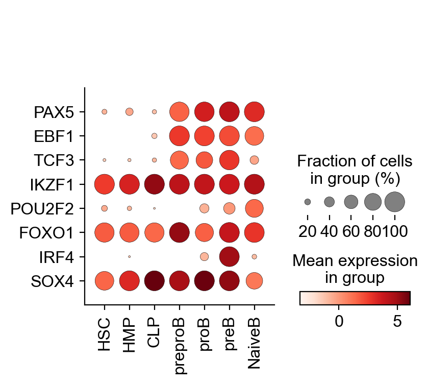
key_TFs = ["PAX5", "EBF1", "TCF3", "IKZF1", "POU2F2", "FOXO1", "IRF4", "SOX4"]
To assess how TF activities are distributed across different cell populations, we can leverage standard scanpy functions like sc.pl.dotplot and sc.pl.violin.
sc.pl.dotplot(
    gdata["GRN"],
    var_names=key_TFs,
    groupby="celltype",
    use_raw=False,
    swap_axes=True,
)
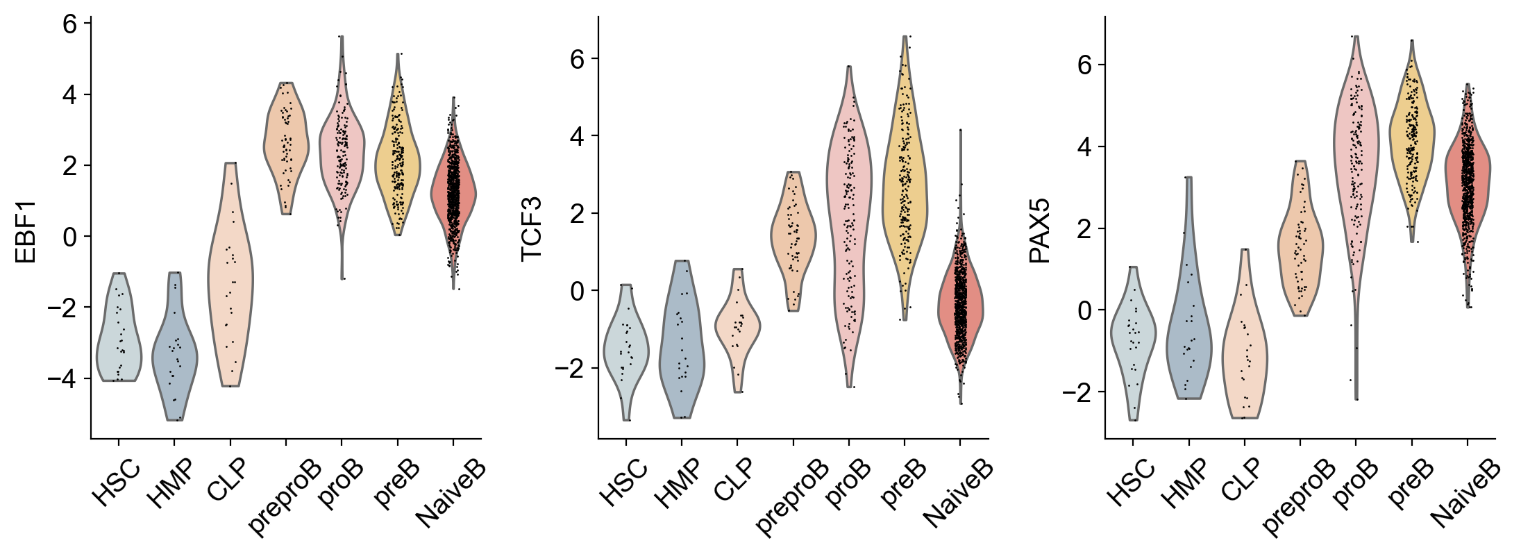
sc.pl.violin(
    gdata["GRN"], keys=["EBF1", "TCF3", "PAX5"], groupby="celltype", use_raw=False, rotation=45, multi_panel=True
)
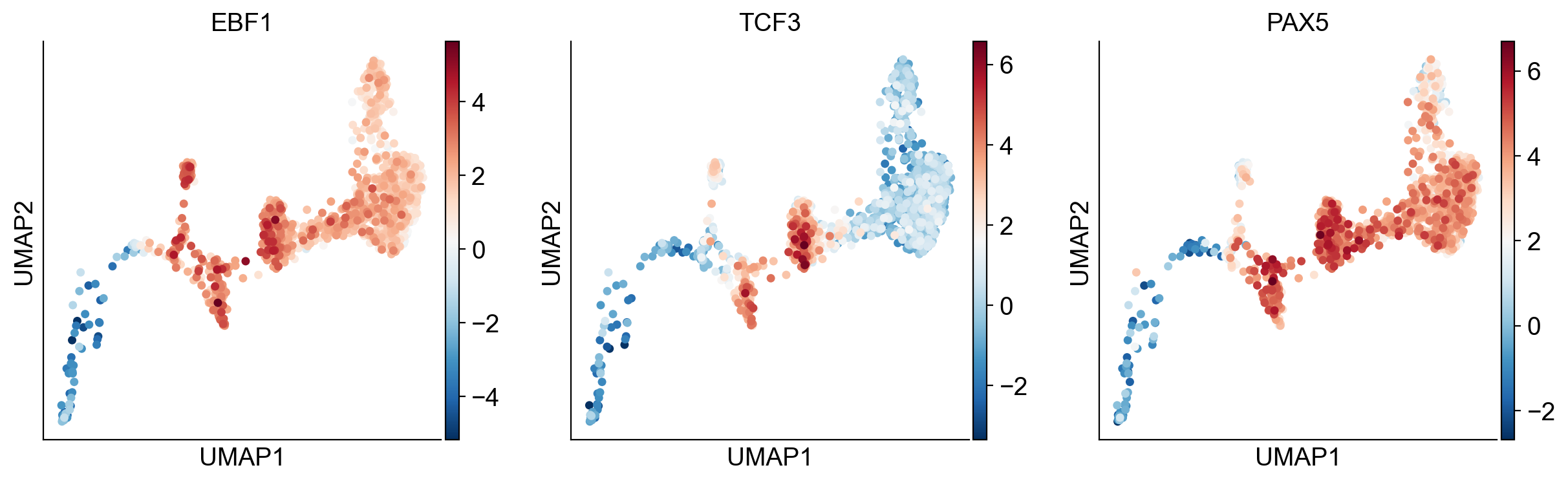
sc.pl.umap(
    gdata["GRN"],
    color=["EBF1", "TCF3", "PAX5"],
    use_raw=False,
    cmap="RdBu_r",
    ncols=3,
)
Finally, scm.pl.trendplot offers a powerful way to directly compare the dynamics of a TF’s regulatory activity (from gdata[“GRN”]) against its own mRNA expression (from gdata[“RNA”]) along the differentiation pseudotime.
scm.pl.trendplot(
    gdata,
    var_dict={"EBF1": [("RNA", "log1p_norm"), ("GRN", None)]},
    normalize=True,
    sortby="palantir_pseudotime",
    col_color=["celltype"],
    palette=["#C53D26", "#CA5A03"],
    figsize=(6, 3),
    dpi=100,
    n_splines=5,
    show_tkey=False,
    show_stds=True,
)
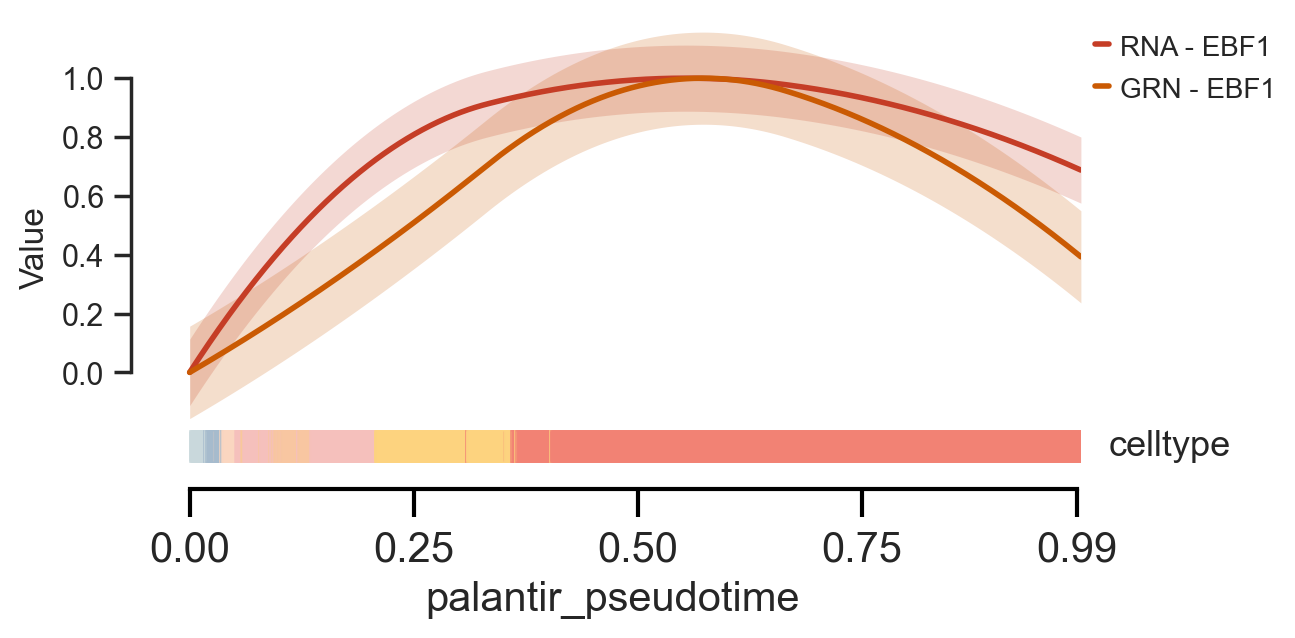
<Axes: xlabel='palantir_pseudotime', ylabel='Value'>
scm.pl.trendplot(
    gdata,
    var_dict={"EBF1": [("GRN", None)], "TCF3": [("GRN", None)], "PAX5": [("GRN", None)]},
    normalize=True,
    sortby="palantir_pseudotime",
    col_color=["celltype"],
    figsize=(6, 3),
    dpi=100,
    n_splines=5,
    show_tkey=False,
    show_stds=True,
)
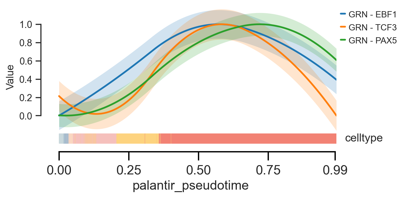
<Axes: xlabel='palantir_pseudotime', ylabel='Value'>
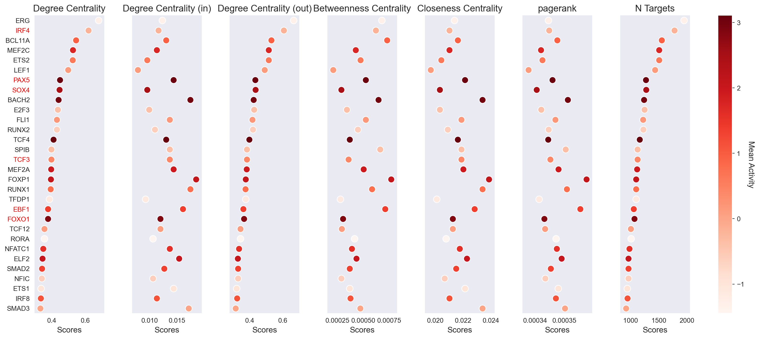
Network Analysis#
Beyond individual TF activities, scMagnify provides tools to analyze the topology of the entire inferred GRN. We can use graph-based network metrics to identify the most central and influential regulators in the system.
The function get_network_score() calculates a suite of standard centrality measures for each TF based on the inferred network structure. This includes:
Degree Centrality (total, in, and out)
Betweenness Centrality
Closeness Centrality
PageRank
Number of Targets (
n_targets)
These scores are computed and stored in gdata["GRN"].varm["network_score"].
gdata = scm.tl.get_network_score(gdata)
gdata["GRN"].varm["network_score"].head()
| degree_centrality | degree_centrality(in) | degree_centrality(out) | betweenness_centrality | closeness_centrality | pagerank | n_targets | |
|---|---|---|---|---|---|---|---|
| AHR | 0.032468 | 0.003418 | 0.029050 | 0.000007 | 0.018391 | 0.000335 | 85 |
| ARID5B | 0.174641 | 0.017088 | 0.157553 | 0.000225 | 0.023396 | 0.000350 | 461 |
| ATF2 | 0.161312 | 0.004101 | 0.157211 | 0.000051 | 0.018300 | 0.000336 | 460 |
| BACH1 | 0.305878 | 0.011620 | 0.294258 | 0.000353 | 0.021123 | 0.000348 | 861 |
| BACH2 | 0.440533 | 0.017430 | 0.423103 | 0.000646 | 0.023396 | 0.000351 | 1238 |
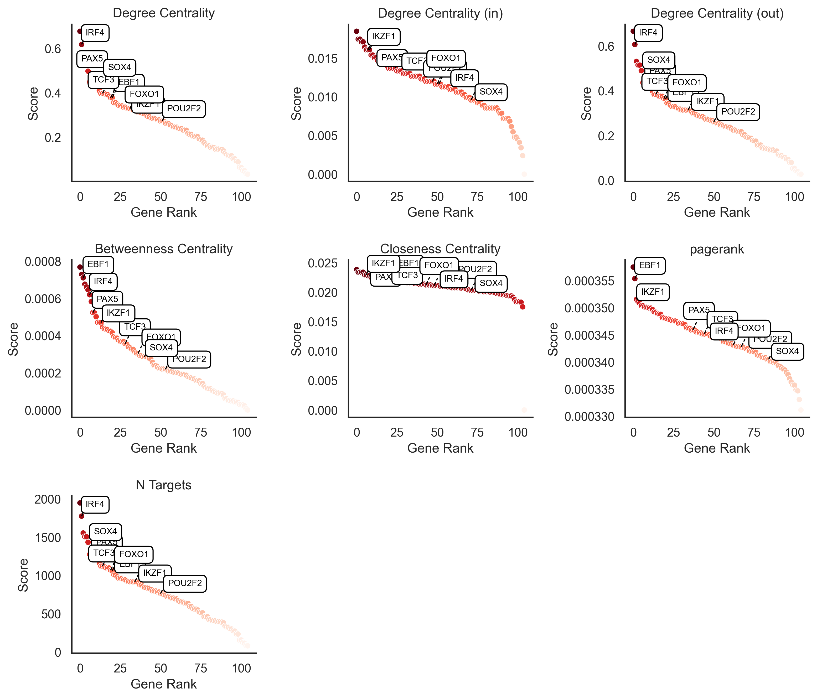
scm.pl.stripplot(gdata, sortby="degree_centrality", selected_genes=key_TFs)
scm.pl.rankplot(gdata, selected_genes=key_TFs, show=True)
Save the data#
gdata.write(os.path.join(settings.data_dir, "gdata_tcelldep-bm_03_NaiveB.h5mu"))
Closing matters#
What’s next?#
In this tutorial, you learned how to infer the multi-scale GRN using scm.MAGNI. This produced a GRNMuData object containing the inferred network, TF regulatory activities, and network centrality scores, allowing you to identify key individual regulators.
However, TFs often work in combination. For the next steps, we recommend the following:
Proceed to the final tutorial on RegFactor Decomposition and Enrichment. This analysis will allow you to move beyond individual TFs and discover combinatorial “modules” of co-regulating TFs using tensor decomposition.
Refer to the API to explore the available parameter values that can be used to customize these computations for your data.
If you encounter any bugs or have suggestions for new features, please open an issue. For general questions, please post on the scverse discourse or contact us at chenxufeng2022@sinh.ac.cn.
Package versions#
import session_info

session_info.show()
Click to view session information
-----
matplotlib          3.10.5
mudata              0.2.3
numba               0.61.2
numpy               1.26.4
pandas              2.3.1
scanpy              1.10.3
scmagnify           0.0.0
seaborn             0.13.2
session_info        v1.0.1
-----
Click to view modules imported as dependencies
MOODS                       NA
PIL                         11.3.0
PyComplexHeatmap            1.8.2
SEACells                    0.3.3
adjustText                  1.3.0
anndata                     0.9.2
anyio                       NA
appdirs                     1.4.4
arrow                       1.3.0
asttokens                   NA
attr                        25.3.0
attrs                       25.3.0
babel                       2.17.0
backports                   NA
biothings_client            0.4.1
cellrank                    2.0.7
certifi                     2025.08.03
cffi                        1.17.1
charset_normalizer          3.4.2
click                       8.2.1
colorama                    0.4.6
comm                        0.2.3
cycler                      0.12.1
cython_runtime              NA
dateutil                    2.9.0.post0
debugpy                     1.8.17
decorator                   5.2.1
decoupler                   2.1.1
defusedxml                  0.7.1
deprecated                  1.2.18
dill                        0.4.0
diskcache                   5.6.3
docrep                      0.3.2
exceptiongroup              1.3.0
executing                   2.2.1
fastjsonschema              NA
filelock                    3.18.0
fqdn                        NA
genomepy                    0.16.1
grandalf                    NA
h5py                        3.14.0
httpx                       0.28.1
idna                        3.10
igraph                      0.11.9
ipykernel                   6.30.1
ipywidgets                  8.1.7
isoduration                 NA
jaraco                      NA
jax                         0.6.2
jaxlib                      0.6.2
jedi                        0.19.2
jinja2                      3.1.6
joblib                      1.5.1
json5                       0.12.0
jsonpointer                 3.0.0
jsonschema                  4.25.0
jsonschema_specifications   NA
jupyter_events              0.12.0
jupyter_server              2.16.0
jupyterlab_server           2.27.3
kiwisolver                  1.4.8
lark                        1.2.2
legacy_api_wrap             NA
legendkit                   0.3.6
llvmlite                    0.44.0
loguru                      0.7.3
markupsafe                  3.0.2
marsilea                    0.5.4
matplotlib_inline           0.1.7
ml_dtypes                   0.5.3
more_itertools              10.3.0
mpl_toolkits                NA
mpmath                      1.3.0
mygene                      3.2.2
mysql                       NA
natsort                     8.4.0
nbformat                    5.10.4
ncls                        NA
netgraph                    4.13.2
networkx                    3.4.2
norns                       NA
nvfuser                     NA
nvidia                      NA
opt_einsum                  3.4.0
overrides                   NA
packaging                   25.0
palantir                    1.4.1
palettable                  3.3.3
parso                       0.8.5
patsy                       1.0.1
petsc4py                    3.23.4
pexpect                     4.9.0
pkg_resources               NA
platformdirs                4.5.0
plotly                      6.3.0
pooch                       v1.8.2
progressbar                 4.5.0
prometheus_client           NA
prompt_toolkit              3.0.52
psutil                      7.1.0
ptyprocess                  0.7.0
pure_eval                   0.2.3
pyarrow                     20.0.0
pycparser                   2.22
pydev_ipython               NA
pydevconsole                NA
pydevd                      3.2.3
pydevd_file_utils           NA
pydevd_plugins              NA
pydevd_tracing              NA
pyfaidx                     0.8.1.4
pygam                       0.10.1
pygments                    2.19.2
pygpcca                     1.0.4
pynndescent                 0.5.13
pyparsing                   3.2.3
pyranges                    0.1.4
pysam                       0.23.1
python_utils                NA
pythonjsonlogger            NA
pytz                        2025.2
referencing                 NA
requests                    2.32.4
rfc3339_validator           0.1.4
rfc3986_validator           0.1.1
rfc3987_syntax              NA
rich                        NA
rpack                       2.0.4
rpds                        NA
scipy                       1.15.3
scvelo                      0.3.3
send2trash                  NA
simplejson                  3.20.1
six                         1.17.0
sklearn                     1.5.2
slepc4py                    3.23.2
sniffio                     1.3.1
sorted_nearest              0.0.39
sphinxcontrib               NA
stack_data                  0.6.3
statsmodels                 0.14.5
swig_runtime_data4          NA
sympy                       1.14.0
tensorly                    0.9.0
texttable                   1.7.0
threadpoolctl               3.6.0
torch                       2.0.0+cu117
tornado                     6.5.2
tqdm                        4.67.1
traitlets                   5.14.3
typing_extensions           NA
umap                        0.5.7
uri_template                NA
urllib3                     2.5.0
vscode                      NA
wcwidth                     0.2.14
webcolors                   NA
websocket                   1.8.0
wrapt                       1.17.2
yaml                        6.0.2
zmq                         27.1.0
zoneinfo                    NA
-----
IPython             8.37.0
jupyter_client      8.6.3
jupyter_core        5.8.1
jupyterlab          4.4.5
-----
Python 3.10.18 | packaged by conda-forge | (main, Jun  4 2025, 14:45:41) [GCC 13.3.0]
Linux-5.14.0-503.31.1.el9_5.x86_64-x86_64-with-glibc2.34
-----
Session information updated at 2025-10-28 08:48