RegFactor Decomposition with scMagnify#
Preliminaries#
In this tutorial, you will learn how to:
RegFactor Decomposition. Decipher the combinatorial effects of transcription factors (TFs) using tensor decomposition.
Enrichment Analysis. Perform gene functional enrichment analysis based on the resulting Regulons.
The Rationale for Decomposition#
In the previous steps, we inferred a GRN and identified key individual regulators. However, it is well-established that TFs rarely act alone; they typically function in a combinatorial manner to orchestrate complex gene expression programs [].
To systematically explore these regulatory synergies, scMagnify implements a RegFactor Decomposition module. This approach is built upon a modified Tucker decomposition, a powerful technique from tensor analysis.
Instead of decomposing raw expression, this method is applied directly to a tensor constructed from the regulatory coefficients (Reg. scores) generated by our multi-scale Granger causality model. This allows the decomposition to focus purely on the inferred regulatory logic.
The primary goal is to simultaneously identify:
Co-regulating TF modules (groups of TFs that function as a unit).
Shared sets of Target Genes (TGs) that are controlled by these modules across different time lags.
This analysis elevates our understanding from individual TF-TG links to the higher-order “teams” of regulators driving the cellular process.
For a complete theoretical breakdown of the tensor decomposition method and the model mathematics, please refer to the [About the MSNGC](./About the MSNGC.md) section and the Methods section of our manuscript.
Import packages#
%load_ext autoreload
%autoreload 2
import warnings
from numba.core.errors import NumbaDeprecationWarning

warnings.simplefilter("ignore", category=NumbaDeprecationWarning)
warnings.simplefilter("ignore", FutureWarning)
warnings.simplefilter("ignore", UserWarning)
warnings.simplefilter("ignore", RuntimeWarning)
import os

import matplotlib.pyplot as plt
import scanpy as sc
import decoupler as dc
import scmagnify as scm
import scmagnify.logging as logg
from scmagnify.settings import settings
scm.info()
 |
|
Configurations#
scm.settings.verbosity = 2
%matplotlib inline

scm.settings.set_figure_params(
    dpi=100,
    facecolor="white",
    frameon=False,
)

scm.load_fonts(["Arial"])
plt.rcParams["font.family"] = "Arial"
plt.rcParams["grid.alpha"] = 0
# Setting a workspace
dirPjtHome = "/mnt/TrueNas/project/chenxufeng/Data/PMID36973557_NatBiotechnol2023_T-cell-depleted/"
workDir = os.path.join(dirPjtHome, "scmagnify_wd")
scm.set_workspace(workDir)
workspace: /mnt/TrueNas/project/chenxufeng/Data/PMID36973557_NatBiotechnol2023_T-cell-depleted/scmagnify_wd/
├── data
├── models
├── tmpfiles
└── figures
# Set up Reference Genome
scm.set_genome(version="hg38", genomes_dir="/home/chenxufeng/picb_cxf/Ref/human/hg38/")
                        Genome Information
┏━━━━━━━━━┳━━━━━━━━━━┳━━━━━━━━━━━━━━━━━━━━━━━━━━━━━━━━━━━━━━━━━━━┓
┃ Version ┃ Provider ┃ Directory                                 ┃
┡━━━━━━━━━╇━━━━━━━━━━╇━━━━━━━━━━━━━━━━━━━━━━━━━━━━━━━━━━━━━━━━━━━┩
│ hg38    │ UCSC     │ /home/chenxufeng/picb_cxf/Ref/human/hg38/ │
└─────────┴──────────┴───────────────────────────────────────────┘
Load the data#
gdata = scm.read(os.path.join(settings.data_dir, "t-cell-depleted-bm_NaiveB_final.h5mu"))
RegFactor Decomposition#
The decomposition workflow is a straightforward, multi-step process.
First, we initialize the RegDecomp object from our gdata. This class automatically extracts the regulatory coefficient tensor and prepares it for decomposition.
decomper = scm.RegDecomp(gdata)
INFO Initializing RegDecomp object with multiscale mode.
INFO     Filtering Network:
          Method: quantile
          Parameter: 0.0
          Binarize: False
Next, we run the tucker_decomposition() method. This is the core step where the tensor is factorized. The rank parameter is critical, as it defines the number of components (RegFactors) to identify. The log output confirms the tensor shape and the Normalized Reconstruction Error (NRE), which measures how well the decomposition approximates the original data.
decomper.tucker_decomposition(rank=5)
INFO     RegFactor Decomposing with Tucker decomposition:
          Tensor shape: (5, 105, 2926)
          Rank: 5
INFO Decomposition NRE: 0.82133766130817
Once the RegFactors (TF modules and their TG sets) are defined, we compute an activity score for each factor in each cell. This is done using the decoupler mlm method, parallel to the individual TF activity calculation.
decomper.compute_activity()
By default, factors are named numerically. We can use rename_regfactors() to re-order or rename them for better biological interpretation in downstream plots.
decomper.rename_regfactors(
    {
        "RegFactor_1": "RegFactor_3",
        "RegFactor_2": "RegFactor_5",
        "RegFactor_3": "RegFactor_4",
        "RegFactor_4": "RegFactor_1",
        "RegFactor_5": "RegFactor_2",
    },
    sort=True,
)
INFO Sorting RegFactors alphabetically.
INFO     Renaming RegFactors: {'RegFactor_1': 'RegFactor_3', 'RegFactor_2': 'RegFactor_5', 'RegFactor_3':
         'RegFactor_4', 'RegFactor_4': 'RegFactor_1', 'RegFactor_5': 'RegFactor_2'}
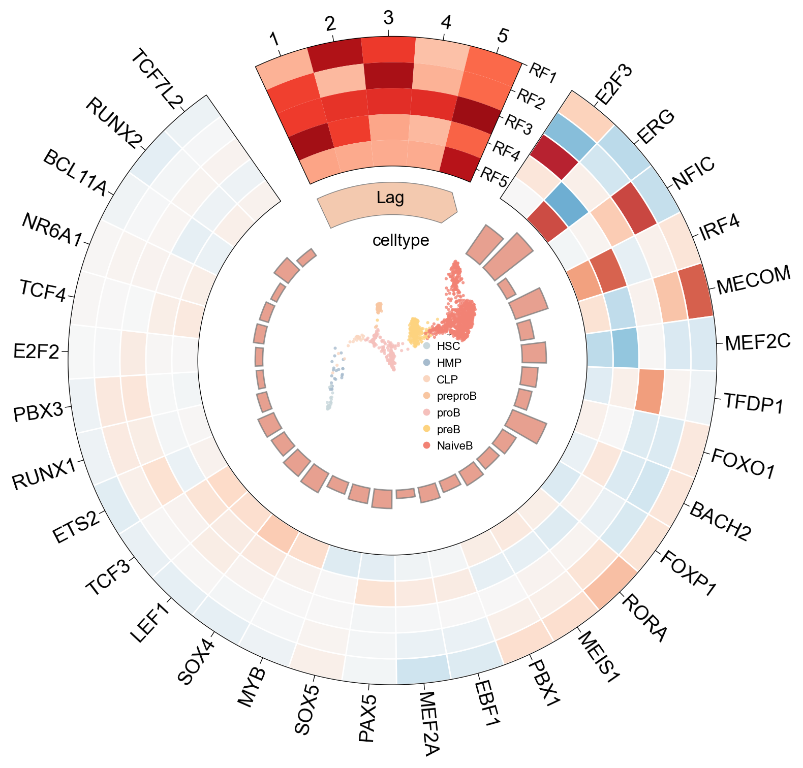
The circosplot() function provides a comprehensive, all-in-one visualization of the decomposition results. This plot effectively summarizes the key components of the inferred regulatory modules:
Outer Ring: The top transcription factors (TFs) that contribute most significantly to each RegFactor.
Inner Heatmap: The time lag associated with each RegFactor.
Center Plot: An embedding (specified by
embedding_key) colored by a cell annotation (specified bycolor_key).
scm.pl.circosplot(
    gdata,
    top_tfs=30,
    cluster=True,
    colorbar=False,
    label_kws={"label_size": 14},
    embedding_key="X_umap",
    color_key="celltype",
    center_axes_rect=(0.40, 0.46, 0.20, 0.20),
)
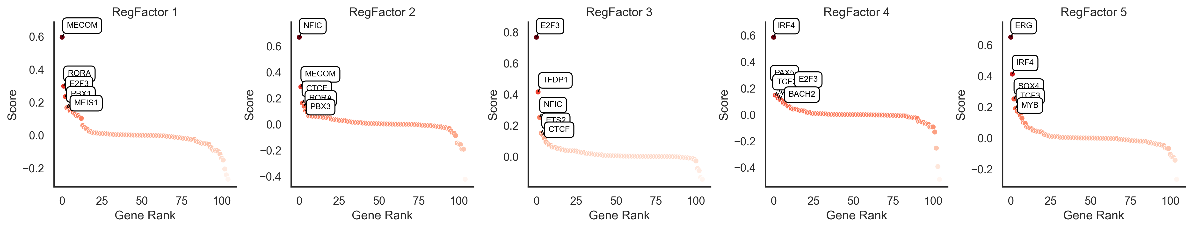
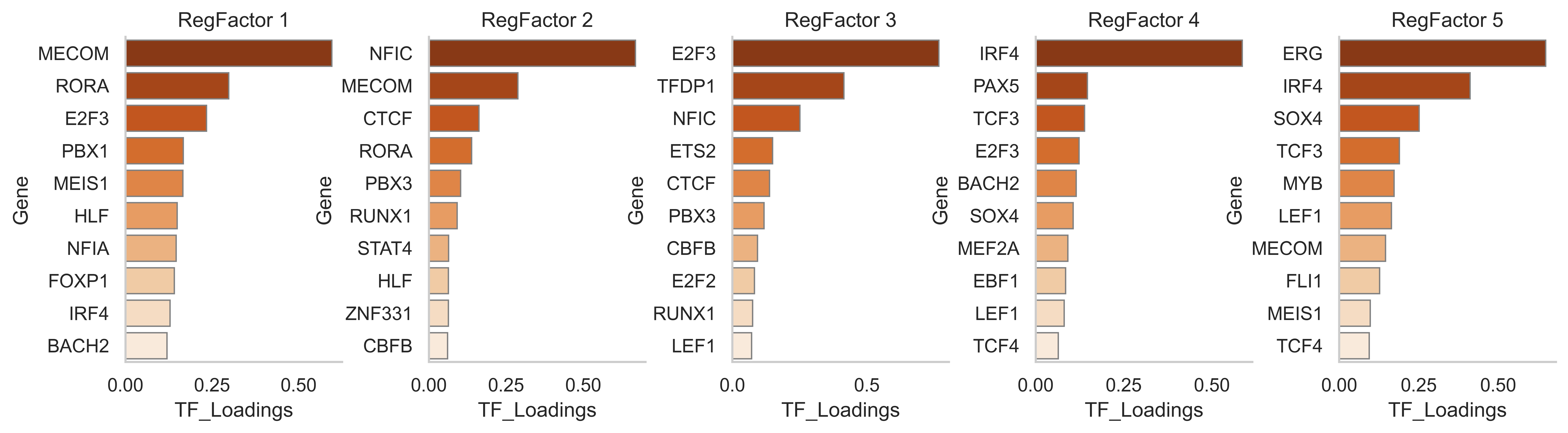
TF Loadings#
The “TF loadings” represent the contribution score of each transcription factor to a given RegFactor module. We can visualize these scores to understand the composition of each module.
scm.pl.rankplot(
    gdata,
    modal="RegFactor",
    key="TF_loadings",
    cmap="Reds",
    n_top=5,
    ncols=5,
    wspace=0.3,
    swap_df=True,
    figsize=(20, 3),
    show=True,
)
scm.pl.barplot(
    gdata, modal="RegFactor", key="TF_loadings", swap_df=True, n_top=10, ncols=5, cmap="Oranges_r", xlabel="TF_Loadings"
)
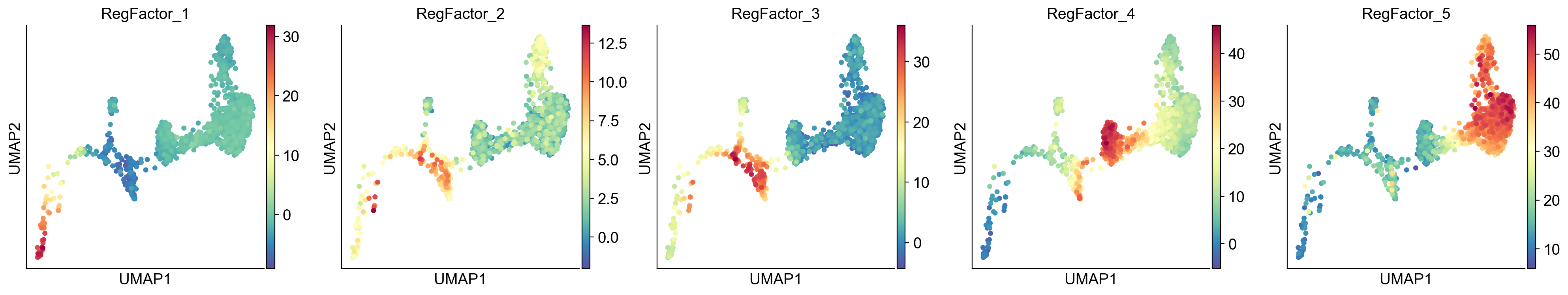
RegFactor Activity#
The activity of each RegFactor represents the combined regulatory influence of its constituent TFs. This activity is computed for each cell and stored in gdata["RegFactor"]. We can visualize these activities just like individual TF activities.
sc.pl.umap(gdata["RegFactor"], color=gdata["RegFactor"].var_names, ncols=5, cmap="Spectral_r")
sc.pl.violin(gdata["RegFactor"], groupby="celltype", keys=gdata["RegFactor"].var_names, rotation=90)
Finally, we can use scm.pl.trendplot to visualize the dynamic changes in RegFactor activity over pseudotime, allowing us to see when each regulatory module is turned “on” or “off” during the differentiation process.
scm.pl.trendplot(
    gdata,
    var_dict={
        "RegFactor_1": [("RegFactor", None)],
        "RegFactor_2": [("RegFactor", None)],
        "RegFactor_3": [("RegFactor", None)],
        "RegFactor_4": [("RegFactor", None)],
        "RegFactor_5": [("RegFactor", None)],
    },
    normalize=True,
    sortby="palantir_pseudotime",
    col_color=["celltype"],
    figsize=(6, 3),
    dpi=100,
    n_splines=5,
    show_tkey=False,
    show_stds=False,
)
<Axes: xlabel='palantir_pseudotime', ylabel='Value'>
Funch Enrich#
To understand the biological functions of the identified RegFactors, we can perform a functional enrichment analysis on their target gene sets. scMagnify implements a standard Over-Representation Analysis (ORA) for this purpose.
First, we can define a color palette for our RegFactors, which will be used in subsequent plots.
gdata.uns["regfactors_colors"] = ["#CED7DA", "#AFBAC9", "#E6C8C3", "#E6CF8C", "#D49284"]
from scmagnify.tools import FuncEnrich
Next, we initialize the {py:class}~scmagnify.tools.FuncEnrich object. We specify the gene set database to use—in this case, the human MSigDB (v2025.1) gene symbols. We then filter this comprehensive database to include only the “Gene Ontology Biological Process” (GOBP) terms.
enricher = FuncEnrich(gene_sets="msigdb.v2025.1.Hs.symbols")
enricher.filter_genesets(pattern="GOBP")
INFO Initializing FuncEnrich object.
INFO     Loading built-in gene set: msigdb.v2025.1.Hs.symbols from
         /home/chenxufeng/WorkSpace/Git-repos/scMagnify/src/scmagnify/data/genesets/msigdb.v2025.1.Hs.symbols.gmt
INFO Successfully loaded 35134 gene sets with a total of 43351 unique gene symbols.
INFO Filtering 35134 gene sets with pattern: 'GOBP'.
INFO Filter applied. Kept 7583 of 35134 gene sets.
tg_dict = scm.tl.extract_regfactor_genes(
    gdata,
    mode="TG",
    plot=True,
    n_top=500,
)
     RegFactor Gene Summary
┏━━━━━━━━━━━━━┳━━━━━━━━━━━━━━━━━┓
┃ RegFactor   ┃ Number of Genes ┃
┡━━━━━━━━━━━━━╇━━━━━━━━━━━━━━━━━┩
│ RegFactor_1 │             500 │
│ RegFactor_2 │             500 │
│ RegFactor_3 │             500 │
│ RegFactor_4 │             500 │
│ RegFactor_5 │             500 │
└─────────────┴─────────────────┘
enr_pvals_dict = {}
regfactors_to_process = list(tg_dict.keys())  # Create a list to iterate over

for regfactor in regfactors_to_process:
    logg.info(f"Running ORA for regfactor: [bold cyan]{regfactor}[/bold cyan]")
    top_genes = tg_dict[regfactor].index

    # Use the run_ora method from the initialized object.
    # For best results, set n_background to the total number of genes
    # detected in your experiment (e.g., len(adata.var_names)).
    enr_pvals = enricher.run_ora(
        gene_list=top_genes,
        n_background=20000,  # Recommended: Replace with your actual background size
        top_n_results=10,  # Show top 5 results in the console summary
    )

    # Store the full results
    enr_pvals_dict[regfactor] = enr_pvals

    # Check if the results DataFrame is not empty before plotting
    if enr_pvals.empty:
        logg.warning(f"No enrichment results found for {regfactor}. Skipping plot.")
        continue

    # Filter for significant results
    enr_pvals_fil = enr_pvals[enr_pvals["FDR p-value"] < 0.05]

    # Check if any significant terms remain after filtering
    if enr_pvals_fil.empty:
        logg.warning(f"No significant terms (FDR < 0.05) for {regfactor}. Skipping plot.")
        continue

    # Create the dot plot for the top 30 significant terms
    dc.pl.dotplot(
        enr_pvals_fil.sort_values("Combined score", ascending=False).head(30),
        x="Combined score",
        y="Term",
        s="Odds ratio",
        c="FDR p-value",
        cmap="viridis",
        scale=0.1,
        figsize=(3, 6),
    )
    plt.title(regfactor)
    plt.show()
INFO Running ORA for regfactor: RegFactor_1
INFO Starting ORA for a list of 500 genes.
INFO Using a user-defined background size of 20000 genes.
                                     Top 10 Enriched Terms
┏━━━━━━━━━━━━━━━━━━━━━━━━━━━━━━━━━━━━━━━━━━━━━━━━━━━━┳━━━━━━━━━┳━━━━━━━━━━━━━━━━┳━━━━━━━━━━━━━┓
┃ Term                                               ┃ Overlap ┃ Combined score ┃ FDR p-value ┃
┡━━━━━━━━━━━━━━━━━━━━━━━━━━━━━━━━━━━━━━━━━━━━━━━━━━━━╇━━━━━━━━━╇━━━━━━━━━━━━━━━━╇━━━━━━━━━━━━━┩
│ GOBP_SPHINGOLIPID_TRANSLOCATION                    │   4/5   │       4.34e+02 │    3.68e-04 │
│ GOBP_POSITIVE_REGULATION_OF_FC_RECEPTOR_MEDIATED_… │   3/6   │       1.76e+02 │    1.31e-02 │
│ GOBP_EMBRYONIC_HEMOPOIESIS                         │  7/24   │       1.67e+02 │    3.23e-04 │
│ GOBP_PLATELET_ACTIVATING_FACTOR_METABOLIC_PROCESS  │   3/8   │       1.18e+02 │    2.59e-02 │
│ GOBP_NEGATIVE_REGULATION_OF_SMOOTH_MUSCLE_CONTRAC… │  4/14   │       1.01e+02 │    1.38e-02 │
│ GOBP_PRIMITIVE_HEMOPOIESIS                         │   3/9   │       1.00e+02 │    3.18e-02 │
│ GOBP_LYMPHOCYTE_DIFFERENTIATION                    │ 39/440  │       9.70e+01 │    3.22e-08 │
│ GOBP_POSITIVE_REGULATION_OF_MAST_CELL_PROLIFERATI… │   2/5   │       9.35e+01 │    9.62e-02 │
│ GOBP_NUCLEAR_MIGRATION_ALONG_MICROTUBULE           │   2/5   │       9.35e+01 │    9.62e-02 │
│ GOBP_REGULATION_OF_CELL_DIFFERENTIATION_INVOLVED_… │   2/5   │       9.35e+01 │    9.62e-02 │
└────────────────────────────────────────────────────┴─────────┴────────────────┴─────────────┘
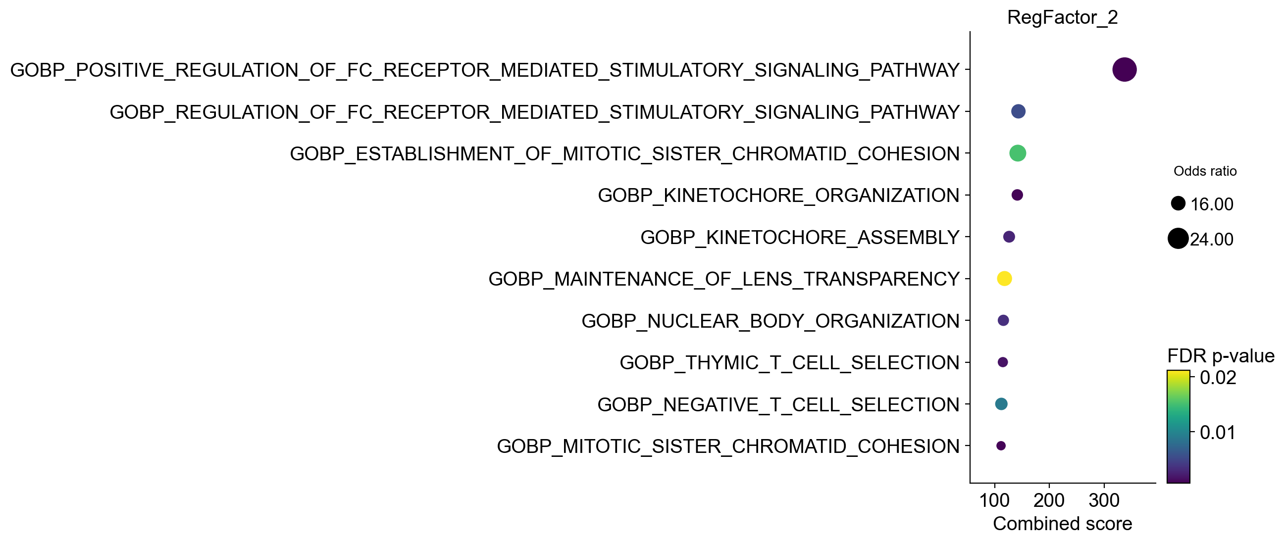
INFO Running ORA for regfactor: RegFactor_2
INFO Starting ORA for a list of 500 genes.
INFO Using a user-defined background size of 20000 genes.
                                     Top 10 Enriched Terms
┏━━━━━━━━━━━━━━━━━━━━━━━━━━━━━━━━━━━━━━━━━━━━━━━━━━━━┳━━━━━━━━━┳━━━━━━━━━━━━━━━━┳━━━━━━━━━━━━━┓
┃ Term                                               ┃ Overlap ┃ Combined score ┃ FDR p-value ┃
┡━━━━━━━━━━━━━━━━━━━━━━━━━━━━━━━━━━━━━━━━━━━━━━━━━━━━╇━━━━━━━━━╇━━━━━━━━━━━━━━━━╇━━━━━━━━━━━━━┩
│ GOBP_POSITIVE_REGULATION_OF_FC_RECEPTOR_MEDIATED_… │   4/6   │       3.37e+02 │    6.16e-04 │
│ GOBP_REGULATION_OF_FC_RECEPTOR_MEDIATED_STIMULATO… │  4/11   │       1.43e+02 │    5.43e-03 │
│ GOBP_ESTABLISHMENT_OF_MITOTIC_SISTER_CHROMATID_CO… │   3/7   │       1.42e+02 │    1.52e-02 │
│ GOBP_KINETOCHORE_ORGANIZATION                      │  6/21   │       1.41e+02 │    7.85e-04 │
│ GOBP_KINETOCHORE_ASSEMBLY                          │  5/17   │       1.27e+02 │    2.72e-03 │
│ GOBP_MAINTENANCE_OF_LENS_TRANSPARENCY              │   3/8   │       1.18e+02 │    2.12e-02 │
│ GOBP_NUCLEAR_BODY_ORGANIZATION                     │  5/18   │       1.16e+02 │    3.39e-03 │
│ GOBP_THYMIC_T_CELL_SELECTION                       │  6/24   │       1.15e+02 │    1.63e-03 │
│ GOBP_NEGATIVE_T_CELL_SELECTION                     │  4/13   │       1.12e+02 │    9.04e-03 │
│ GOBP_MITOTIC_SISTER_CHROMATID_COHESION             │  7/31   │       1.12e+02 │    7.84e-04 │
└────────────────────────────────────────────────────┴─────────┴────────────────┴─────────────┘
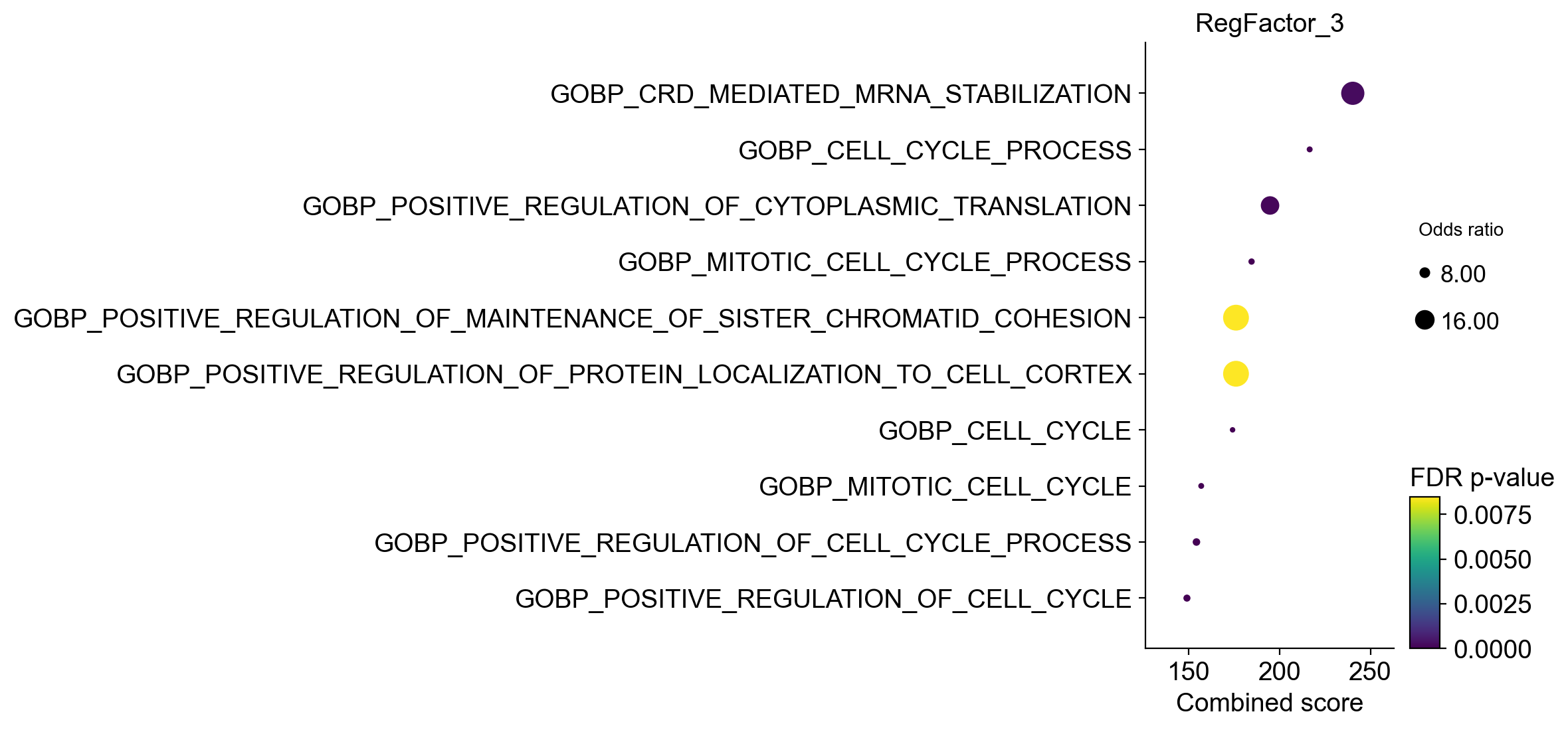
INFO Running ORA for regfactor: RegFactor_3
INFO Starting ORA for a list of 500 genes.
INFO Using a user-defined background size of 20000 genes.
                                     Top 10 Enriched Terms
┏━━━━━━━━━━━━━━━━━━━━━━━━━━━━━━━━━━━━━━━━━━━━━━━━━━━━┳━━━━━━━━━━┳━━━━━━━━━━━━━━━━┳━━━━━━━━━━━━━┓
┃ Term                                               ┃ Overlap  ┃ Combined score ┃ FDR p-value ┃
┡━━━━━━━━━━━━━━━━━━━━━━━━━━━━━━━━━━━━━━━━━━━━━━━━━━━━╇━━━━━━━━━━╇━━━━━━━━━━━━━━━━╇━━━━━━━━━━━━━┩
│ GOBP_CRD_MEDIATED_MRNA_STABILIZATION               │   5/11   │       2.40e+02 │    2.54e-04 │
│ GOBP_CELL_CYCLE_PROCESS                            │ 105/1348 │       2.17e+02 │    1.29e-22 │
│ GOBP_POSITIVE_REGULATION_OF_CYTOPLASMIC_TRANSLATI… │   6/17   │       1.95e+02 │    1.65e-04 │
│ GOBP_MITOTIC_CELL_CYCLE_PROCESS                    │  70/783  │       1.85e+02 │    1.47e-17 │
│ GOBP_POSITIVE_REGULATION_OF_PROTEIN_LOCALIZATION_… │   3/6    │       1.76e+02 │    8.46e-03 │
│ GOBP_POSITIVE_REGULATION_OF_MAINTENANCE_OF_SISTER… │   3/6    │       1.76e+02 │    8.46e-03 │
│ GOBP_CELL_CYCLE                                    │ 116/1705 │       1.74e+02 │    1.08e-20 │
│ GOBP_MITOTIC_CELL_CYCLE                            │  75/931  │       1.57e+02 │    1.75e-16 │
│ GOBP_POSITIVE_REGULATION_OF_CELL_CYCLE_PROCESS     │  33/275  │       1.54e+02 │    2.72e-11 │
│ GOBP_POSITIVE_REGULATION_OF_CELL_CYCLE             │  38/346  │       1.49e+02 │    8.71e-12 │
└────────────────────────────────────────────────────┴──────────┴────────────────┴─────────────┘
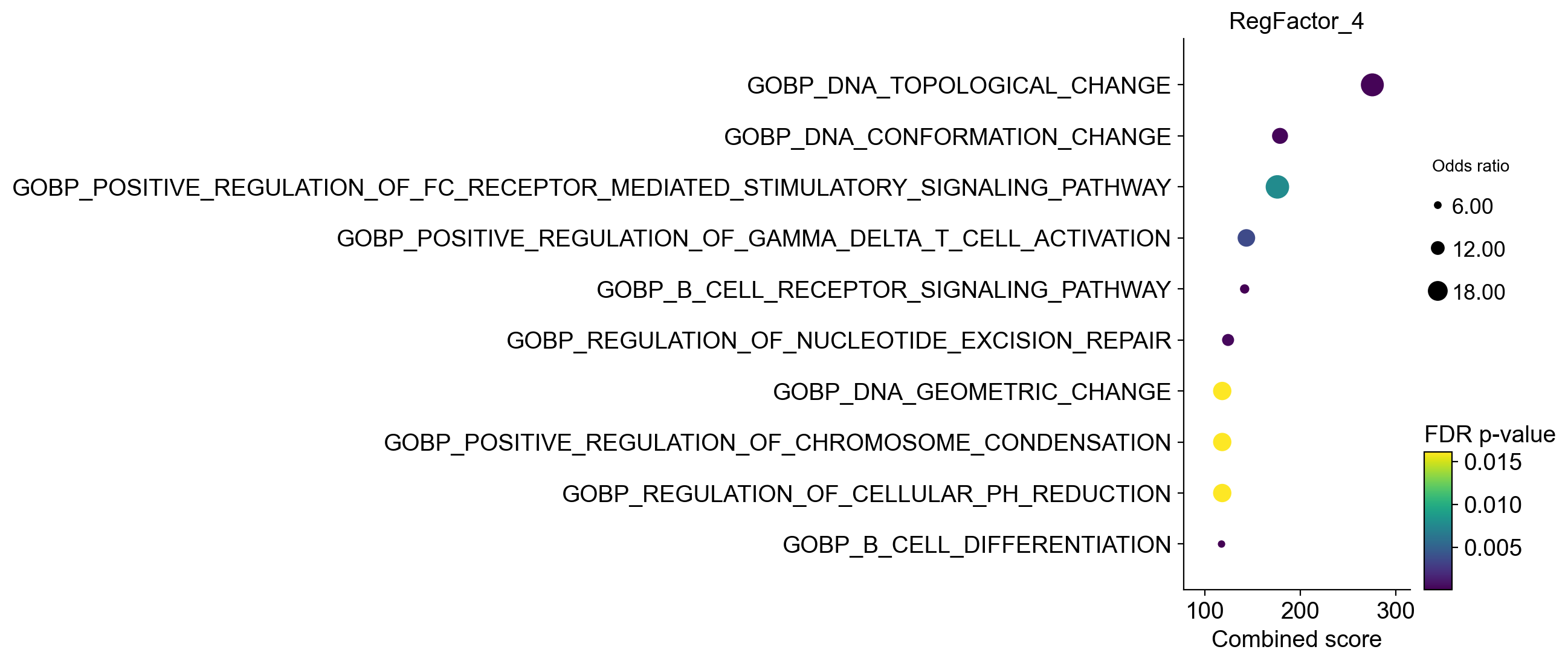
INFO Running ORA for regfactor: RegFactor_4
INFO Starting ORA for a list of 500 genes.
INFO Using a user-defined background size of 20000 genes.
                                     Top 10 Enriched Terms
┏━━━━━━━━━━━━━━━━━━━━━━━━━━━━━━━━━━━━━━━━━━━━━━━━━━━━┳━━━━━━━━━┳━━━━━━━━━━━━━━━━┳━━━━━━━━━━━━━┓
┃ Term                                               ┃ Overlap ┃ Combined score ┃ FDR p-value ┃
┡━━━━━━━━━━━━━━━━━━━━━━━━━━━━━━━━━━━━━━━━━━━━━━━━━━━━╇━━━━━━━━━╇━━━━━━━━━━━━━━━━╇━━━━━━━━━━━━━┩
│ GOBP_DNA_TOPOLOGICAL_CHANGE                        │  5/10   │       2.76e+02 │    1.54e-04 │
│ GOBP_DNA_CONFORMATION_CHANGE                       │  6/18   │       1.79e+02 │    2.27e-04 │
│ GOBP_POSITIVE_REGULATION_OF_FC_RECEPTOR_MEDIATED_… │   3/6   │       1.76e+02 │    7.69e-03 │
│ GOBP_POSITIVE_REGULATION_OF_GAMMA_DELTA_T_CELL_AC… │  4/11   │       1.43e+02 │    3.62e-03 │
│ GOBP_B_CELL_RECEPTOR_SIGNALING_PATHWAY             │  14/78  │       1.42e+02 │    1.64e-06 │
│ GOBP_REGULATION_OF_NUCLEOTIDE_EXCISION_REPAIR      │  7/29   │       1.24e+02 │    3.39e-04 │
│ GOBP_REGULATION_OF_CELLULAR_PH_REDUCTION           │   3/8   │       1.18e+02 │    1.61e-02 │
│ GOBP_POSITIVE_REGULATION_OF_CHROMOSOME_CONDENSATI… │   3/8   │       1.18e+02 │    1.61e-02 │
│ GOBP_DNA_GEOMETRIC_CHANGE                          │   3/8   │       1.18e+02 │    1.61e-02 │
│ GOBP_B_CELL_DIFFERENTIATION                        │ 20/149  │       1.17e+02 │    2.82e-07 │
└────────────────────────────────────────────────────┴─────────┴────────────────┴─────────────┘
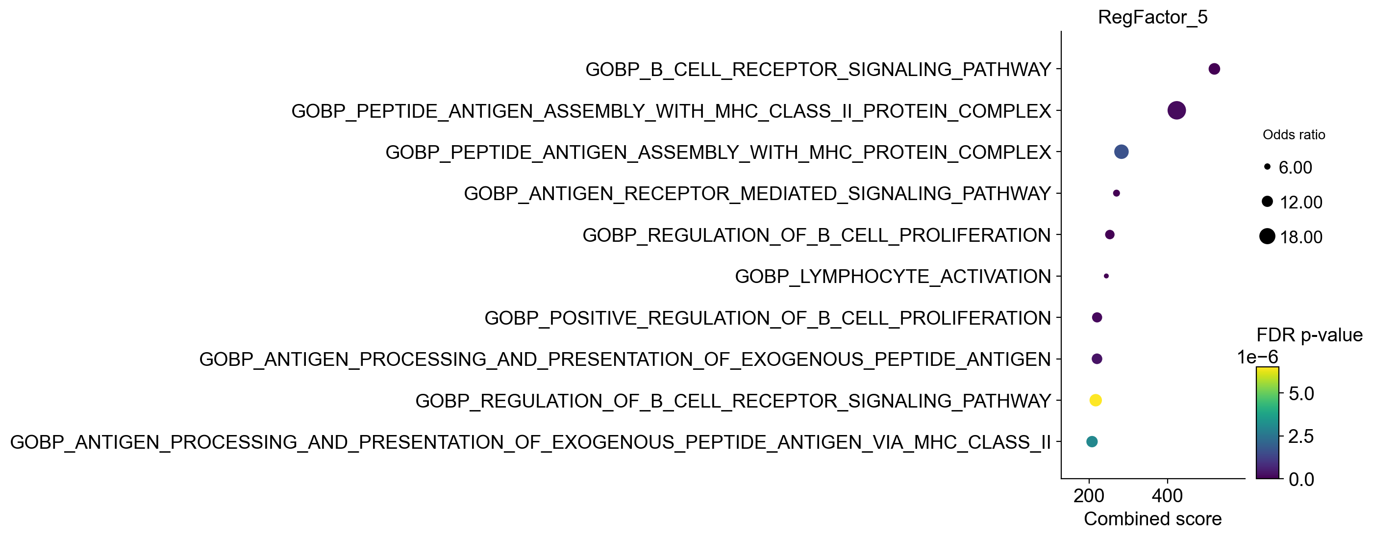
INFO Running ORA for regfactor: RegFactor_5
INFO Starting ORA for a list of 500 genes.
INFO Using a user-defined background size of 20000 genes.
                                     Top 10 Enriched Terms
┏━━━━━━━━━━━━━━━━━━━━━━━━━━━━━━━━━━━━━━━━━━━━━━━━━━━━┳━━━━━━━━━┳━━━━━━━━━━━━━━━━┳━━━━━━━━━━━━━┓
┃ Term                                               ┃ Overlap ┃ Combined score ┃ FDR p-value ┃
┡━━━━━━━━━━━━━━━━━━━━━━━━━━━━━━━━━━━━━━━━━━━━━━━━━━━━╇━━━━━━━━━╇━━━━━━━━━━━━━━━━╇━━━━━━━━━━━━━┩
│ GOBP_B_CELL_RECEPTOR_SIGNALING_PATHWAY             │  23/78  │       5.20e+02 │    8.95e-16 │
│ GOBP_PEPTIDE_ANTIGEN_ASSEMBLY_WITH_MHC_CLASS_II_P… │  8/16   │       4.24e+02 │    1.64e-07 │
│ GOBP_PEPTIDE_ANTIGEN_ASSEMBLY_WITH_MHC_PROTEIN_CO… │  8/21   │       2.83e+02 │    1.64e-06 │
│ GOBP_ANTIGEN_RECEPTOR_MEDIATED_SIGNALING_PATHWAY   │ 34/214  │       2.70e+02 │    3.64e-15 │
│ GOBP_REGULATION_OF_B_CELL_PROLIFERATION            │  16/68  │       2.53e+02 │    1.06e-09 │
│ GOBP_LYMPHOCYTE_ACTIVATION                         │ 80/846  │       2.44e+02 │    1.47e-21 │
│ GOBP_POSITIVE_REGULATION_OF_B_CELL_PROLIFERATION   │  12/47  │       2.21e+02 │    1.33e-07 │
│ GOBP_ANTIGEN_PROCESSING_AND_PRESENTATION_OF_EXOGE… │  11/41  │       2.20e+02 │    3.28e-07 │
│ GOBP_REGULATION_OF_B_CELL_RECEPTOR_SIGNALING_PATH… │  8/25   │       2.17e+02 │    6.51e-06 │
│ GOBP_ANTIGEN_PROCESSING_AND_PRESENTATION_OF_EXOGE… │  9/31   │       2.08e+02 │    3.05e-06 │
└────────────────────────────────────────────────────┴─────────┴────────────────┴─────────────┘
Network Visualization#
from scmagnify.plotting import GRNVisualizer
custom_term_dict = {
    "GOBP_B_CELL_RECEPTOR_SIGNALING_PATHWAY": [
        "LYN",
        "PTPRC",
        "IGHM",
        "PRKCB",
        "BLK",
        "IGKC",
        "GRB2",
        "FOXP1",
        "NFKB1",
    ],
    "GOBP_B_CELL_DIFFERENTIATION": ["PAX5", "PTPRJ", "PTPRC", "IKZF3", "IGHM", "HDAC9", "CARD11"],
    "GOBP_CHROMATIN_REMODELING": [
        "CHD7",
        "NCOA3",
        "HDAC9",
        "SMCHD1",
        "PRKCB",
        "ATAD2",
        "SETBP1",
        "PCGF5",
        "LBR",
        "DPF3",
    ],
    "GOBP_DNA_TOPOLOGICAL_CHANGE": ["TOP2A", "TOP2B", "HGMB1", "HGMB2"],
}
tf_list = ["EBF1", "PAX5", "IRF4", "TCF3", "SOX4"]
tg_list = tg_list = (
    gdata["RegFactor"].varm["TG_loadings"].T.sort_values(by="RegFactor_4", ascending=False).head(100).index
)
# get tg from custom terms
tg_list = []
for _term, genes in custom_term_dict.items():
    tg_list.extend(genes)
vis = GRNVisualizer(gdata)
vis.prepare_network(regulon=None, tf_list=tf_list, tg_list=tg_list, add_suffixes=True, target_clusters=custom_term_dict)
INFO Building base TF-peak-gene triplet network...
INFO Filtering triplet network using 'network' from gdata.uns...
INFO Base network constructed with 91074 TF-peak-gene relationships.
INFO Filtering network based on provided TF and/or Target Gene lists...
INFO Final network contains 155 relationships after filtering.
INFO Using provided manual target gene clusters.
         Manual Target Gene Clusters Summary
┏━━━━━━━━━━━━━━━━━━━━━━━━━━━━━━━━━━━━━━━━┳━━━━━━━━━━━┓
┃ Cluster                                ┃ Num Genes ┃
┡━━━━━━━━━━━━━━━━━━━━━━━━━━━━━━━━━━━━━━━━╇━━━━━━━━━━━┩
│ GOBP_B_CELL_RECEPTOR_SIGNALING_PATHWAY │ 8         │
│ GOBP_B_CELL_DIFFERENTIATION            │ 6         │
│ GOBP_CHROMATIN_REMODELING              │ 10        │
└────────────────────────────────────────┴───────────┘
<scmagnify.plotting._grn_visualizer.GRNVisualizer at 0x7f44800e48b0>
vis.add_continuous_mapping(
    node_type="TF",
    visual_property="size",
    modal="GRN",  # Assumes gdata has a modal named 'activity'
    varm_key=("network_score", "degree_centrality"),
    map_range=(8, 12),  # Map sizes from 8 to 25
    legend_title="Degree Centrality",
)
INFO Added continuous mapping for 'TF' node 'size'.
<scmagnify.plotting._grn_visualizer.GRNVisualizer at 0x7f44800e48b0>
vis.add_continuous_mapping(
    node_type="Target",
    visual_property="color",
    modal="RNA",  # Assumes gdata has a modal named 'activity'
    map_range="Reds",
    layer="log1p_norm",
    legend_title="RNA Expression",
)
INFO Added continuous mapping for 'Target' node 'color'.
<scmagnify.plotting._grn_visualizer.GRNVisualizer at 0x7f44800e48b0>
vis.r_tf = 0.5
vis.r_ccre = 0.8
vis.r_target = 1.3
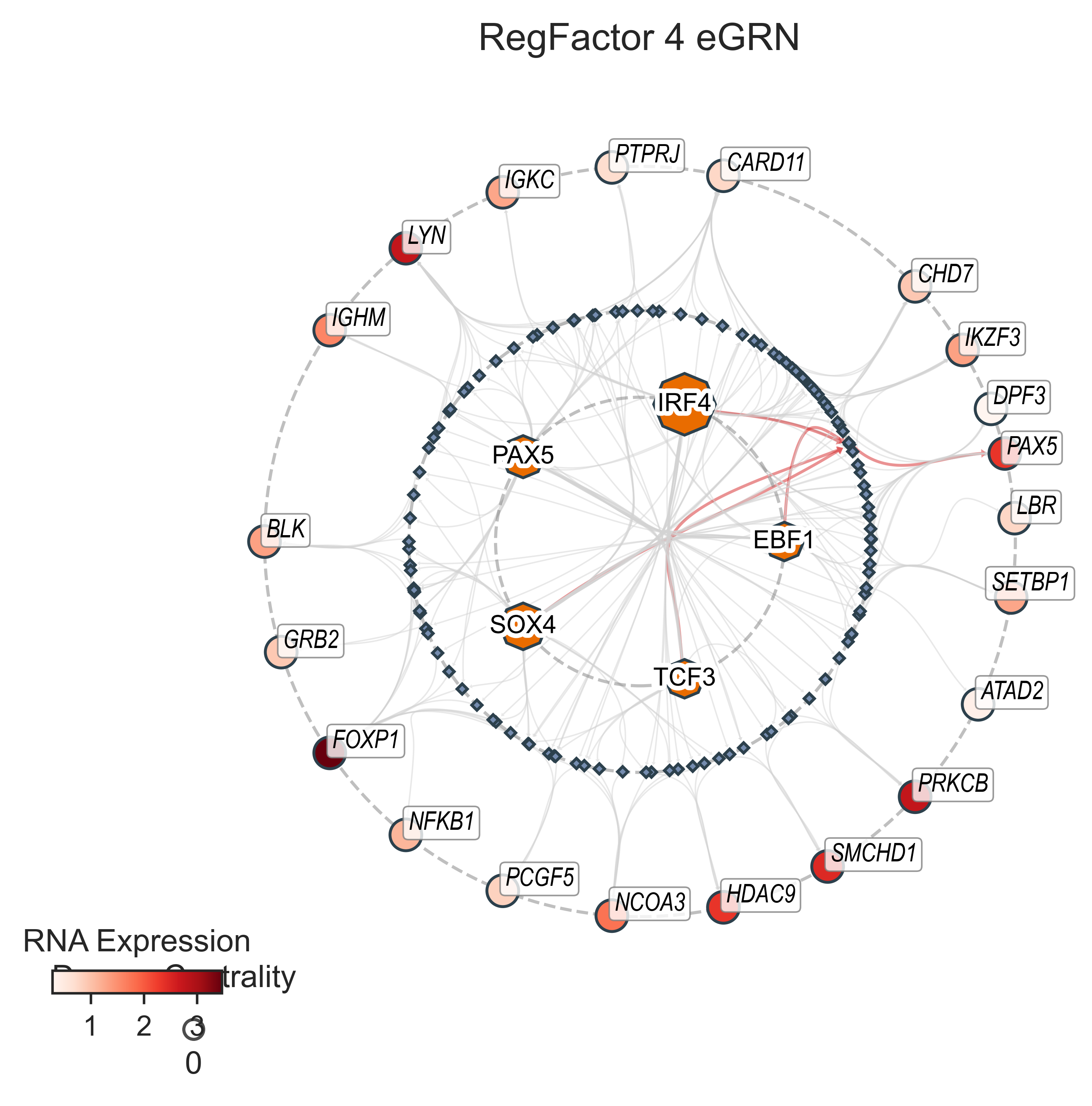
vis.plot(
    figsize=(5, 5),
    dpi=300,
    title="RegFactor 4 eGRN",
    title_fontsize=12,
    node_label_offset=0.2,
    node_edge_width=1,
    tf_layout_mode="uniform",
    label_offset_factor=1,
    label_mode="external",
    edge_layout="bundled",
    highlight={"Target": ["PAX5"], "cCRE": ["chr9:37029184-37029684"], "TF": ["EBF1", "TCF3", "PAX5", "IRF4", "SOX4"]},
    interactive=False,
    jitter_strength=5,
    draw_cluster_wedges=False,
)
INFO Calculating Network Layout...
INFO Applying highlighting to specified nodes and edges...
INFO Applying custom continuous mappings...
Adjusting 21 external target labels to prevent overlap...
Genomic Viewer#
from scmagnify.plotting import GenomeViewer
fragment_files = {
    "IM-1393_BoneMarrow_TcellDep_1_multiome": "/mnt/TrueNas/project/chenxufeng//Data/PMID36973557_NatBiotechnol2023_T-cell-depleted/0_cellranger/BM_Tcelldep_Rep1_atac_fragments.tsv.gz",
    "IM-1393_BoneMarrow_TcellDep_2_multiome": "/mnt/TrueNas/project/chenxufeng//Data/PMID36973557_NatBiotechnol2023_T-cell-depleted/0_cellranger/BM_Tcelldep_Rep2_atac_fragments.tsv.gz",
}
viewer = GenomeViewer(data=gdata, modal="ATAC", fragment_files=fragment_files, cluster="celltype")
INFO Attempting to auto-load peaks from 'ATAC' modality's .var_names...
INFO ✅ Successfully auto-loaded 216477 peaks as 'Peaks'.
INFO Attempting to auto-load links from gdata.uns['peak_gene_corrs']['filtered_corrs']...
INFO ✅ Successfully auto-loaded 22745 links from gdata.
INFO Preprocessing metadata...
INFO Loading and processing GTF...
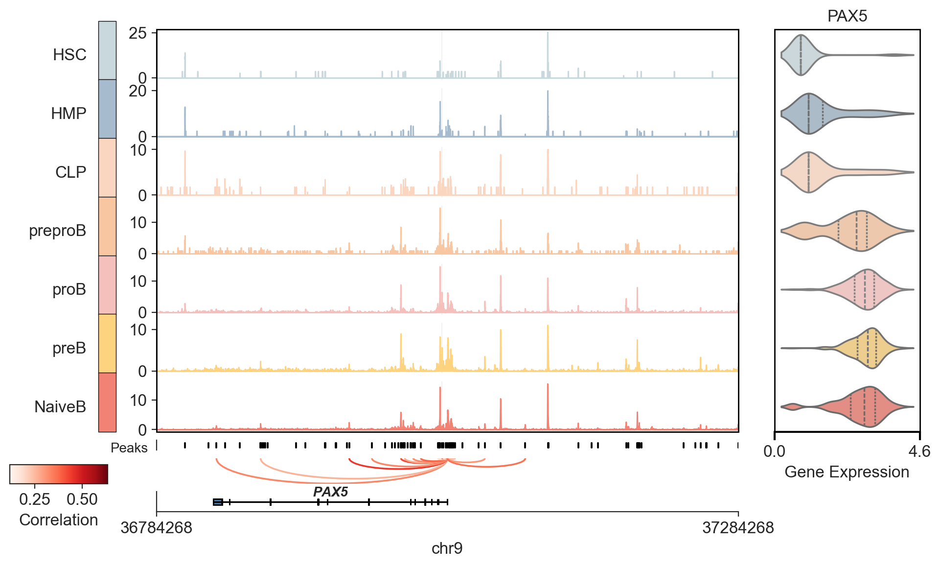
viewer.plot(
    anchor_gene="PAX5",
    theme="ticks",
    side_genes=["PAX5"],
    anchor_flank=250000,
    normalize=True,
    show_motif_logos=False,
    rasterize_coverage=True,
    highlight_peaks=["chr9:37029184-37029684"],
)
INFO Processing peaks for highlighting...
INFO                             peak  gene       cor      pval chrom     start  \
         5731  chr9:36835204-36835704  PAX5  0.417219  0.002627  chr9  36835204
         5732  chr9:36873230-36873730  PAX5  0.280841  0.045795  chr9  36873230
         5733  chr9:36949396-36949896  PAX5  0.633355  0.001788  chr9  36949396
         5734  chr9:36968883-36969383  PAX5  0.407278  0.007072  chr9  36968883
         5735  chr9:36993858-36994358  PAX5  0.586656  0.009581  chr9  36993858
         5736  chr9:36997154-36997654  PAX5  0.304038  0.022332  chr9  36997154
         5737  chr9:37004392-37004892  PAX5  0.397404  0.007143  chr9  37004392
         5738  chr9:37010921-37011421  PAX5  0.513678  0.002850  chr9  37010921
         5739  chr9:37025579-37026079  PAX5  0.132025  0.086116  chr9  37025579
         5740  chr9:37029184-37029684  PAX5  0.443045  0.018797  chr9  37029184
         5741  chr9:37030276-37030776  PAX5  0.118639  0.063281  chr9  37030276
         5742  chr9:37032656-37033156  PAX5  0.383195  0.002373  chr9  37032656
         5743  chr9:37034085-37034585  PAX5  0.404153  0.029794  chr9  37034085
         5744  chr9:37037198-37037698  PAX5  0.137647  0.090633  chr9  37037198
         5745  chr9:37037840-37038340  PAX5  0.403106  0.007047  chr9  37037840
         5746  chr9:37040435-37040935  PAX5  0.248222  0.039122  chr9  37040435
         5747  chr9:37066033-37066533  PAX5  0.362238  0.014985  chr9  37066033
         5748  chr9:37100720-37101220  PAX5  0.475527  0.001061  chr9  37100720

                    end
         5731  36835704
         5732  36873730
         5733  36949896
         5734  36969383
         5735  36994358
         5736  36997654
         5737  37004892
         5738  37011421
         5739  37026079
         5740  37029684
         5741  37030776
         5742  37033156
         5743  37034585
         5744  37037698
         5745  37038340
         5746  37040935
         5747  37066533
         5748  37101220
INFO Plotting 18 links.
INFO Drawing highlights for 1 regions.
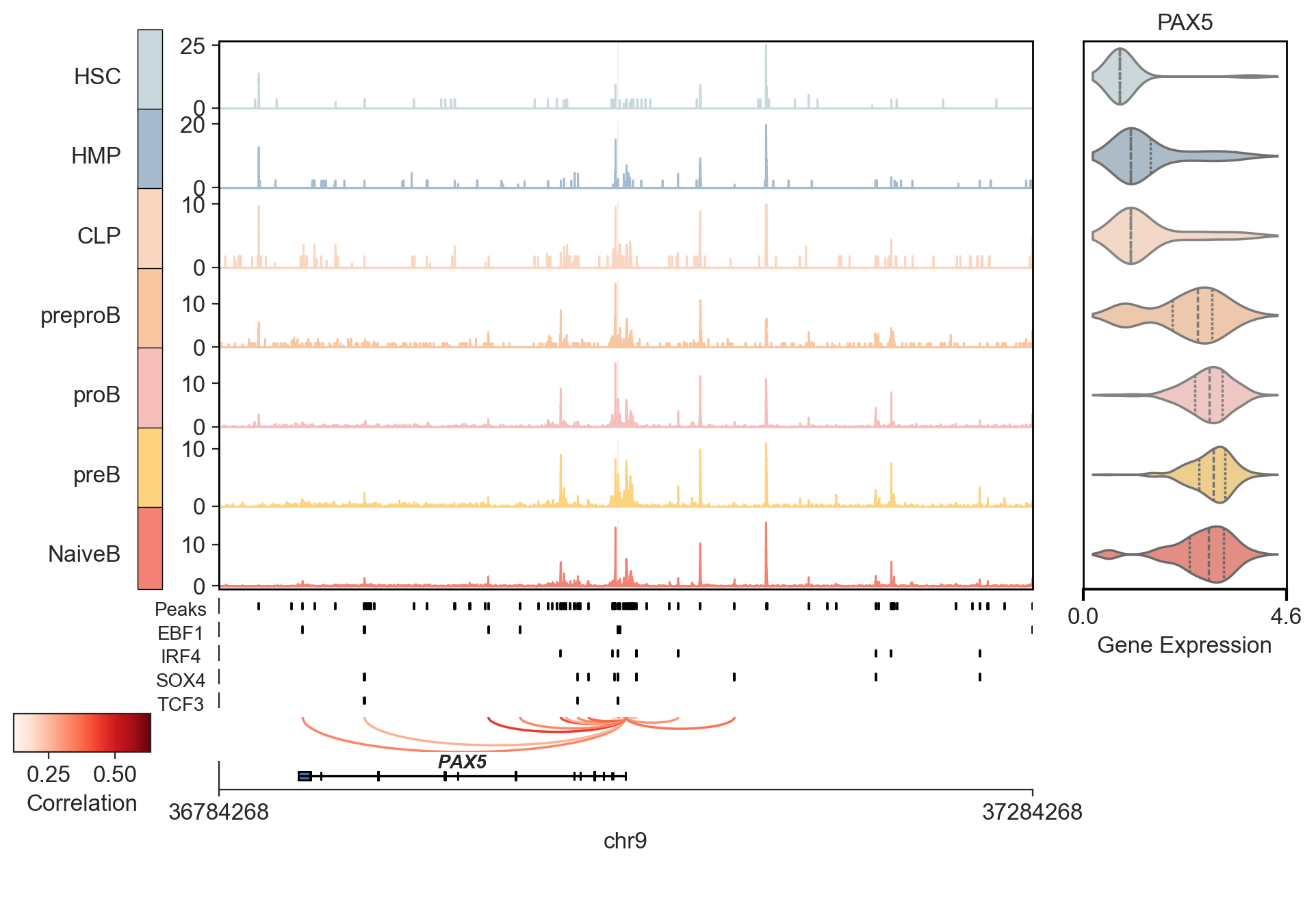
viewer.add_motifs(
    tfs=["EBF1", "IRF4", "SOX4", "TCF3"],
    motif_db="HOCOMOCOv11_HUMAN",
)
INFO Added 4 new motifs. Total motifs: 4.
INFO Added 4 motifs for plotting.
viewer.plot(
    anchor_gene="PAX5",
    theme="ticks",
    side_genes=["PAX5"],
    anchor_flank=250000,
    normalize=True,
    highlight_peaks=["chr9:37029184-37029684"],
    show_motif_logos=False,
    rasterize_coverage=True,
)
INFO Processing peaks for highlighting...
INFO                             peak  gene       cor      pval chrom     start  \
         5731  chr9:36835204-36835704  PAX5  0.417219  0.002627  chr9  36835204
         5732  chr9:36873230-36873730  PAX5  0.280841  0.045795  chr9  36873230
         5733  chr9:36949396-36949896  PAX5  0.633355  0.001788  chr9  36949396
         5734  chr9:36968883-36969383  PAX5  0.407278  0.007072  chr9  36968883
         5735  chr9:36993858-36994358  PAX5  0.586656  0.009581  chr9  36993858
         5736  chr9:36997154-36997654  PAX5  0.304038  0.022332  chr9  36997154
         5737  chr9:37004392-37004892  PAX5  0.397404  0.007143  chr9  37004392
         5738  chr9:37010921-37011421  PAX5  0.513678  0.002850  chr9  37010921
         5739  chr9:37025579-37026079  PAX5  0.132025  0.086116  chr9  37025579
         5740  chr9:37029184-37029684  PAX5  0.443045  0.018797  chr9  37029184
         5741  chr9:37030276-37030776  PAX5  0.118639  0.063281  chr9  37030276
         5742  chr9:37032656-37033156  PAX5  0.383195  0.002373  chr9  37032656
         5743  chr9:37034085-37034585  PAX5  0.404153  0.029794  chr9  37034085
         5744  chr9:37037198-37037698  PAX5  0.137647  0.090633  chr9  37037198
         5745  chr9:37037840-37038340  PAX5  0.403106  0.007047  chr9  37037840
         5746  chr9:37040435-37040935  PAX5  0.248222  0.039122  chr9  37040435
         5747  chr9:37066033-37066533  PAX5  0.362238  0.014985  chr9  37066033
         5748  chr9:37100720-37101220  PAX5  0.475527  0.001061  chr9  37100720

                    end
         5731  36835704
         5732  36873730
         5733  36949896
         5734  36969383
         5735  36994358
         5736  36997654
         5737  37004892
         5738  37011421
         5739  37026079
         5740  37029684
         5741  37030776
         5742  37033156
         5743  37034585
         5744  37037698
         5745  37038340
         5746  37040935
         5747  37066533
         5748  37101220
INFO Plotting 18 links.
INFO Drawing highlights for 1 regions.
Save the Data#
gdata.write(os.path.join(workDir, "gdata_tcelldep-bm_04_NaiveB.h5mu"))
Closing matters#
What’s next?#
In this tutorial, you learned how to use RegDecomp to perform tensor decomposition, identifying combinatorial RegFactors (TF modules) and their target genes. You also learned how to visualize these modules, analyze their activity, and interpret their biological function using enrichment analysis.
This completes the core scMagnify workflow. For your next steps, we recommend:
Applying this workflow to your own data. You can now use this four-part framework to analyze your own single-cell multi-omic datasets from end to end.
Refer to the API to explore all available functions and advanced parameter values that can be used to customize these computations for your specific biological questions.
If you encounter any bugs or have suggestions for new features, please open an issue. For general questions, please post on the scverse discourse or contact us at chenxufeng2022@sinh.ac.cn.
Package versions#
import session_info

session_info.show()
Click to view session information
-----
matplotlib          3.8.4
numba               0.59.1
numpy               1.26.4
pandas              1.5.3
scanpy              1.10.1
scmagnify           NA
seaborn             0.13.2
session_info        1.0.0
-----
Click to view modules imported as dependencies
Bio                         1.83
MOODS                       NA
PIL                         10.3.0
PyComplexHeatmap            1.8.1
absl                        NA
adjustText                  0.8
anndata                     0.9.2
anyio                       NA
appdirs                     1.4.4
argcomplete                 NA
arrow                       1.3.0
asttokens                   NA
attr                        23.2.0
attrs                       23.2.0
babel                       2.15.0
biothings_client            0.3.1
brotli                      1.1.0
cellrank                    2.0.4
certifi                     2024.08.30
cffi                        1.16.0
chardet                     5.2.0
charset_normalizer          3.3.2
chex                        0.1.82
cloudpickle                 3.0.0
colorama                    0.4.6
comm                        0.2.2
contextlib2                 NA
cycler                      0.12.1
cython_runtime              NA
dateutil                    2.9.0.post0
debugpy                     1.8.1
decorator                   5.1.1
defusedxml                  0.7.1
deprecated                  1.2.14
dill                        0.3.8
diskcache                   5.6.3
docrep                      0.3.2
etils                       1.5.2
exceptiongroup              1.2.1
executing                   2.0.1
fastjsonschema              NA
filelock                    3.14.0
flax                        0.7.2
fontTools                   4.51.0
fqdn                        NA
fsspec                      2024.5.0
genomepy                    0.16.1
gmpy2                       2.1.5
h5py                        3.9.0
idna                        3.7
igraph                      0.11.8
importlib_metadata          NA
importlib_resources         NA
ipykernel                   6.29.4
ipywidgets                  8.1.5
isoduration                 NA
jax                         0.4.13
jaxlib                      0.4.13
jedi                        0.19.1
jinja2                      3.0.3
joblib                      1.4.2
json5                       0.10.0
jsonpointer                 3.0.0
jsonschema                  4.22.0
jsonschema_specifications   NA
jupyter_events              0.10.0
jupyter_server              2.14.2
jupyterlab_server           2.27.3
kiwisolver                  1.4.5
legacy_api_wrap             NA
leidenalg                   0.10.2
lightning                   2.1.4
lightning_utilities         0.11.2
llvmlite                    0.42.0
loguru                      0.7.2
louvain                     0.8.2
lxml                        5.3.0
markupsafe                  2.1.5
matplotlib_inline           0.1.7
ml_collections              NA
ml_dtypes                   0.4.0
mpl_toolkits                NA
mpmath                      1.3.0
msgpack                     1.0.8
mudata                      0.2.3
multipledispatch            0.6.0
mygene                      3.2.2
mysql                       NA
natsort                     8.4.0
nbformat                    5.10.4
ncls                        0.0.68
networkx                    3.1
norns                       NA
numexpr                     2.10.0
numpyro                     0.12.1
nvfuser                     NA
opt_einsum                  v3.3.0
optax                       0.2.1
overrides                   NA
packaging                   24.0
palettable                  3.3.3
parso                       0.8.4
patsy                       0.5.6
petsc4py                    3.19.1
pexpect                     4.9.0
pkg_resources               NA
platformdirs                4.2.2
plotly                      5.24.1
progressbar                 4.4.2
prometheus_client           NA
prompt_toolkit              3.0.36
psutil                      5.9.8
ptyprocess                  0.7.0
pure_eval                   0.2.2
pyarrow                     18.0.0
pycirclize                  1.7.2
pycparser                   2.22
pydev_ipython               NA
pydevconsole                NA
pydevd                      2.9.5
pydevd_file_utils           NA
pydevd_plugins              NA
pydevd_tracing              NA
pyfaidx                     0.7.2.2
pygam                       0.9.1
pygments                    2.18.0
pygpcca                     1.0.4
pyparsing                   3.1.2
pyranges                    0.1.1
pyro                        1.9.0+f02dfb9
pysam                       0.22.1
python_utils                NA
pythonjsonlogger            NA
pytz                        2024.2
referencing                 NA
requests                    2.31.0
rfc3339_validator           0.1.4
rfc3986_validator           0.1.1
rich                        NA
rpds                        NA
scipy                       1.12.0
scvelo                      0.3.3.dev3+gf21651c
scvi                        1.1.6
send2trash                  NA
six                         1.16.0
sklearn                     1.5.2
slepc4py                    3.19.1
sniffio                     1.3.1
socks                       1.7.1
sorted_nearest              0.0.39
sparse                      0.15.4
sphinxcontrib               NA
stack_data                  0.6.3
statsmodels                 0.14.2
swig_runtime_data4          NA
sympy                       1.12
tensorly                    0.9.0
texttable                   1.7.0
threadpoolctl               3.5.0
toolz                       0.12.1
torch                       2.0.0+cu118
torchmetrics                1.4.0.post0
tornado                     6.4
tqdm                        4.66.4
traitlets                   5.14.3
typing_extensions           NA
uri_template                NA
urllib3                     2.2.1
wcwidth                     0.2.13
webcolors                   NA
websocket                   1.8.0
wrapt                       1.16.0
yaml                        6.0.1
zipp                        NA
zmq                         26.0.3
zoneinfo                    NA
-----
IPython             8.18.0
jupyter_client      8.6.1
jupyter_core        5.7.2
jupyterlab          4.3.3
notebook            7.3.1
-----
Python 3.9.19 | packaged by conda-forge | (main, Mar 20 2024, 12:50:21) [GCC 12.3.0]
Linux-3.10.0-1160.90.1.el7.x86_64-x86_64-with-glibc2.17
-----
Session information updated at 2025-02-17 00:54