Intracellular Communication Modeling with scMagnify#
Preliminaries#
In this tutorial, you will learn how to:
Cell-cell Communication analysis with LIANA+
Infer Dynamic Signaling-to-Transcription Axes. Correlate receptor expression with intracellular TF activity along a pseudotime trajectory.
Rationale#
Intercellular communication via ligand-receptor (L-R) interactions is fundamental to coordinating cellular responses in development and disease. However, a key challenge is understanding how these extracellular signals are dynamically translated into specific intracellular transcriptional programs to orchestrate cell state transitions [].
To address this, scMagnify provides a dynamic communication module. This analysis moves beyond simple L-R pairing and aims to connect intercellular signaling (receptors) directly to the intracellular TF activity along a defined differentiation trajectory.
Briefly, the workflow first establishes potential ligand-receptor-TF links from a knowledgebase. It then correlates receptor expression with TF activity across metacells ordered by pseudotime. Finally, a permutation test is employed to identify statistically significant and robust signaling-to-transcription axes that change dynamically during the process.
Import packages#
%load_ext autoreload
%autoreload 2
import warnings
from numba.core.errors import NumbaDeprecationWarning

warnings.simplefilter("ignore", category=NumbaDeprecationWarning)
warnings.simplefilter("ignore", FutureWarning)
warnings.simplefilter("ignore", UserWarning)
warnings.simplefilter("ignore", RuntimeWarning)
import os
import pandas as pd
import matplotlib.pyplot as plt
import seaborn as sns
import scanpy as sc
import liana as li
import scmagnify as scm
from scmagnify.settings import settings
scm.info()
 |
|
Configurations#
scm.settings.verbosity = 2
%matplotlib inline

scm.settings.set_figure_params(
    dpi=100,
    facecolor="white",
    frameon=False,
)

scm.load_fonts(["Arial"])

plt.rcParams["font.family"] = "Arial"
plt.rcParams["grid.alpha"] = 0
# Setting a workspace
dirPjtHome = "/mnt/TrueNas/project/chenxufeng/Data/PMID38199997_NatCommun2024"
workDir = os.path.join(dirPjtHome, "scmagnify_wd")
scm.set_workspace(workDir)
workspace: /mnt/TrueNas/project/chenxufeng/Data/PMID38199997_NatCommun2024/scmagnify_wd/
├── data
├── models
├── tmpfiles
└── figures
scm.set_genome(version="hg38", genomes_dir="/home/chenxufeng/picb_cxf/Ref/human/hg38/")
                        Genome Information
┏━━━━━━━━━┳━━━━━━━━━━┳━━━━━━━━━━━━━━━━━━━━━━━━━━━━━━━━━━━━━━━━━━━┓
┃ Version ┃ Provider ┃ Directory                                 ┃
┡━━━━━━━━━╇━━━━━━━━━━╇━━━━━━━━━━━━━━━━━━━━━━━━━━━━━━━━━━━━━━━━━━━┩
│ hg38    │ UCSC     │ /home/chenxufeng/picb_cxf/Ref/human/hg38/ │
└─────────┴──────────┴───────────────────────────────────────────┘
Load the Data#
gdata = scm.read(os.path.join(settings.data_dir, "kidney-injury-tal_H11CORE.h5mu"))
gdata
Gene Regulatory Network (GRN) with 30523 edges.
MuData object with n_obs × n_vars = 8080 × 359416
  uns:	'attention_weights', 'filtered_network', 'motif_scan', 'network', 'peak_gene_corrs', 'regfactors', 'regfactors_colors'
  4 modalities
    RNA:	8080 x 22857
      obs:	'nCount_RNA', 'nFeature_RNA', 'library', 'percent.er', 'percent.mt', 'experiment', 'subclass.l3', 'subclass.l2', 'subclass.l1', 'nCount_ATAC', 'nFeature_ATAC', 'nucleosome_signal', 'nucleosome_percentile', 'TSS.enrichment', 'TSS.percentile', 'Total_fragments', 'FRiP', 'RNA.weight', 'ATAC.weight', 'dpt_pseudotime', 'celltype', 'leiden_res_0.50', 'n_counts', 'SEACell'
      var:	'name', 'n_cells', 'significant_genes', 'highly_variable', 'means', 'dispersions', 'dispersions_norm'
      uns:	'celltype_colors', 'celltype_sizes', 'diffmap_evals', 'draw_graph', 'hvg', 'iroot', 'leiden_res_0.50', 'leiden_res_0.50_colors', 'leiden_res_0.50_sizes', 'library_colors', 'log1p', 'neighbors', 'paga', 'subclass.l1_colors', 'subclass.l2_colors', 'subclass.l2_sizes', 'subclass.l3_colors', 'test_assoc', 'umap'
      obsm:	'X_diffmap', 'X_draw_graph_fa', 'X_lsi', 'X_pca', 'X_phate', 'X_umap', 'padj_mlm', 'score_mlm'
      varm:	'test_assoc_res'
      layers:	'counts', 'log1p_norm'
      obsp:	'connectivities', 'distances'
    ATAC:	8080 x 336500
      obs:	'nCount_RNA', 'nFeature_RNA', 'library', 'percent.er', 'percent.mt', 'experiment', 'subclass.l3', 'subclass.l2', 'subclass.l1', 'nCount_ATAC', 'nFeature_ATAC', 'nucleosome_signal', 'nucleosome_percentile', 'TSS.enrichment', 'TSS.percentile', 'Total_fragments', 'FRiP', 'RNA.weight', 'ATAC.weight', 'SEACell'
      var:	'count', 'percentile', 'AA', 'AC', 'AG', 'AT', 'CA', 'CC', 'CG', 'CT', 'GA', 'GC', 'GG', 'GT', 'TA', 'TC', 'TG', 'TT', 'GC.percent', 'sequence.length'
      uns:	'library_colors', 'neighbors', 'peak_seq', 'subclass.l2_colors', 'subclass.l3_colors', 'umap'
      obsm:	'X_lsi', 'X_pca', 'X_svd', 'X_umap'
      layers:	'counts'
      obsp:	'connectivities', 'distances'
    GRN:	8080 x 54
      obs:	'nCount_RNA', 'nFeature_RNA', 'library', 'percent.er', 'percent.mt', 'experiment', 'subclass.l3', 'subclass.l2', 'subclass.l1', 'nCount_ATAC', 'nFeature_ATAC', 'nucleosome_signal', 'nucleosome_percentile', 'TSS.enrichment', 'TSS.percentile', 'Total_fragments', 'FRiP', 'RNA.weight', 'ATAC.weight', 'dpt_pseudotime', 'celltype', 'leiden_res_0.50', 'n_counts', 'SEACell'
      var:	'mean_activity'
      uns:	'basal_grn', 'celltype_colors', 'celltype_sizes', 'diffmap_evals', 'draw_graph', 'hvg', 'iroot', 'leiden_res_0.50', 'leiden_res_0.50_colors', 'leiden_res_0.50_sizes', 'library_colors', 'log1p', 'neighbors', 'paga', 'subclass.l1_colors', 'subclass.l2_colors', 'subclass.l2_sizes', 'subclass.l3_colors', 'test_assoc', 'umap'
      obsm:	'X_diffmap', 'X_draw_graph_fa', 'X_lsi', 'X_pca', 'X_phate', 'X_umap', 'padj_mlm', 'score_mlm'
      varm:	'network_score'
    RegFactor:	8080 x 5
      obs:	'nCount_RNA', 'nFeature_RNA', 'library', 'percent.er', 'percent.mt', 'experiment', 'subclass.l3', 'subclass.l2', 'subclass.l1', 'nCount_ATAC', 'nFeature_ATAC', 'nucleosome_signal', 'nucleosome_percentile', 'TSS.enrichment', 'TSS.percentile', 'Total_fragments', 'FRiP', 'RNA.weight', 'ATAC.weight', 'dpt_pseudotime', 'celltype', 'leiden_res_0.50', 'n_counts', 'SEACell'
      uns:	'celltype_colors', 'celltype_sizes', 'diffmap_evals', 'draw_graph', 'hvg', 'iroot', 'leiden_res_0.50', 'leiden_res_0.50_colors', 'leiden_res_0.50_sizes', 'library_colors', 'log1p', 'neighbors', 'paga', 'subclass.l1_colors', 'subclass.l2_colors', 'subclass.l2_sizes', 'subclass.l3_colors', 'test_assoc', 'umap'
      obsm:	'X_diffmap', 'X_draw_graph_fa', 'X_lsi', 'X_pca', 'X_phate', 'X_umap', 'padj_mlm', 'score_mlm'
varm: 'Lag_loadings', 'TF_loadings', 'TG_loadings'sc.pl.umap(
gdata["RNA"],
color=["celltype"],
size=10,
frameon=False,
)
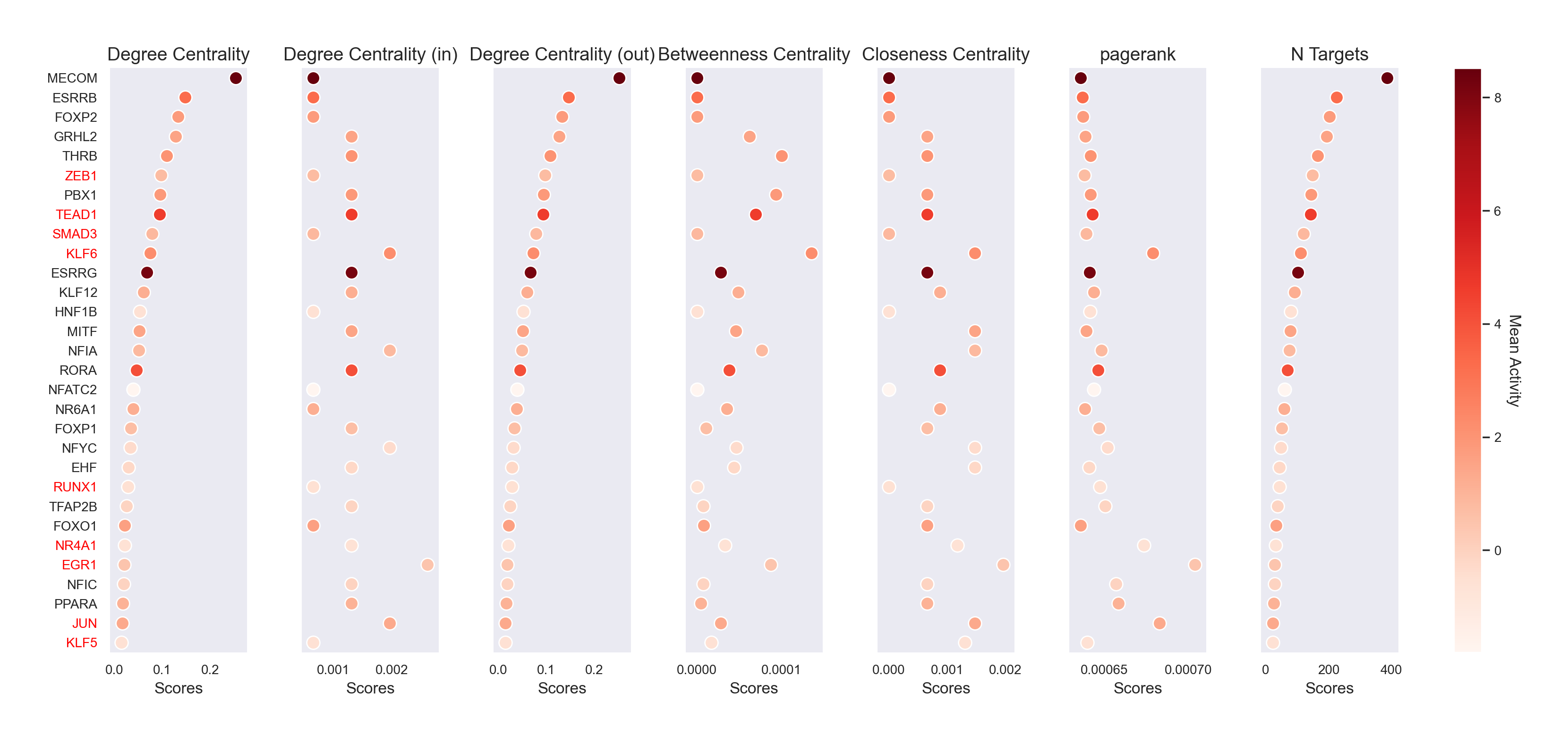
scm.pl.stripplot(gdata, sortby="degree_centrality", n_top=30)
adata_cci = sc.read(
    "/mnt/TrueNas/project/chenxufeng/Data/PMID38199997_NatCommun2024/1_AnnData/kidney-injury-rna_tal_imm.h5ad"
)
adata_cci
AnnData object with n_obs × n_vars = 12813 × 36554
    obs: 'nCount_RNA', 'nFeature_RNA', 'library', 'percent.er', 'percent.mt', 'experiment', 'subclass.l3', 'subclass.l2', 'subclass.l1', 'nCount_ATAC', 'nFeature_ATAC', 'nucleosome_signal', 'nucleosome_percentile', 'TSS.enrichment', 'TSS.percentile', 'Total_fragments', 'FRiP', 'RNA.weight', 'ATAC.weight', 'celltype_hierarchical', 'celltype'
    var: 'name'
    uns: 'celltype_colors', 'dendrogram_celltype_hierarchical', 'library_colors', 'log1p', 'neighbors', 'subclass.l1_colors', 'subclass.l2_colors', 'subclass.l3_colors', 'umap'
    obsm: 'X_lsi', 'X_pca', 'X_umap'
    layers: 'log1p_norm'
    obsp: 'connectivities', 'distances'
sc.pl.umap(adata_cci, color=["celltype", "library", "subclass.l1"], wspace=0.4, ncols=3)
meta_mdata = scm.read(os.path.join(settings.data_dir, "kidney-injury-tal_metacells.h5mu"))
meta_mdata["RNA"].layers["log1p_norm"] = meta_mdata["RNA"].X.copy()
RegFactor Analysis#
scm.pl.barplot(
    gdata,
    modal="RegFactor",
    key="TF_loadings",
    swap_df=True,
    n_top=10,
    ncols=5,
    cmap="Blues_r",
)
scm.pl.barplot(
    gdata,
    modal="RegFactor",
    key="TG_loadings",
    swap_df=True,
    n_top=10,
    ncols=5,
    cmap="Blues_r",
)
sc.pl.violin(
    gdata["RegFactor"], keys=gdata["RegFactor"].var_names, groupby="celltype", rotation=45, stripplot=False, show=True
)
Cell-cell Communication with Liana+#
li.mt.cellchat(
    adata_cci,
    groupby="celltype",
    resource_name="cellchatdb",
    verbose=True,
    use_raw=False,
    layer="log1p_norm",
    key_added="cellchat_res",
)

cellchat_res = adata_cci.uns["cellchat_res"].copy()
Generating ligand-receptor stats for 12813 samples and 878 features
from scmagnify.external.plotting.liana import LianaVisualizer
lvis = LianaVisualizer(
    adata_cci, res_key="cellchat_res", magnitude_col="lr_probs", pvalue_col="cellchat_pvals", cluster_key="celltype"
)
fig = lvis.plot_chord(
    kind="count", normalize="row", link_kws={"ec": "black", "lw": 0, "direction": 1}, label_kws={"size": 15}
)
fig, ax = lvis.plot_interact_heatmap(cmap="Reds")
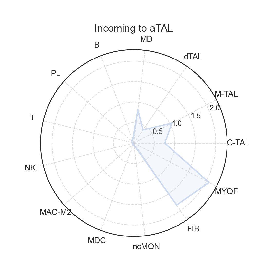
fig, ax = lvis.plot_radar(cell="aTAL", mode="incoming", kind="strength")
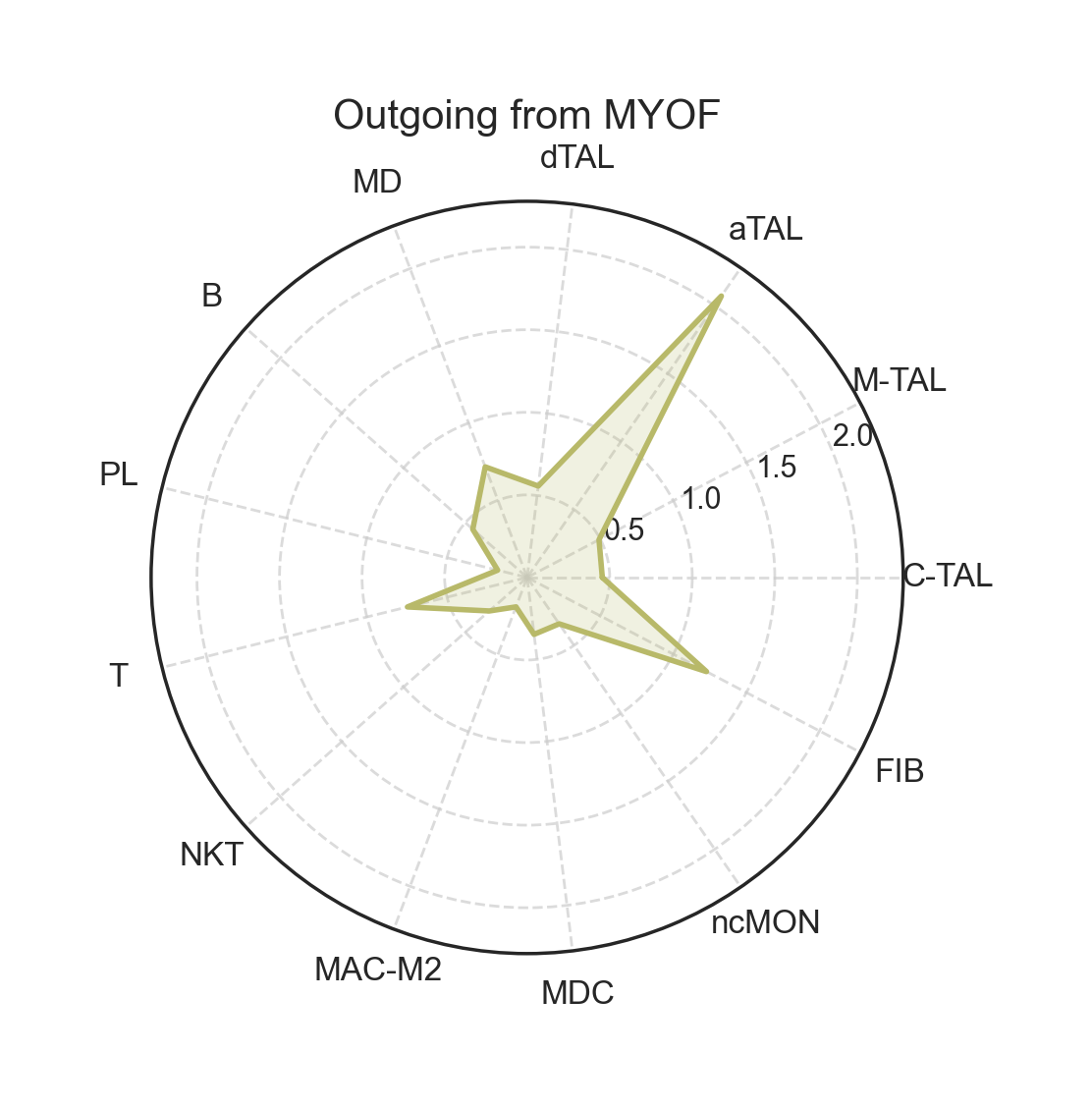
fig, ax = lvis.plot_radar(cell="MYOF", mode="outgoing", kind="strength")
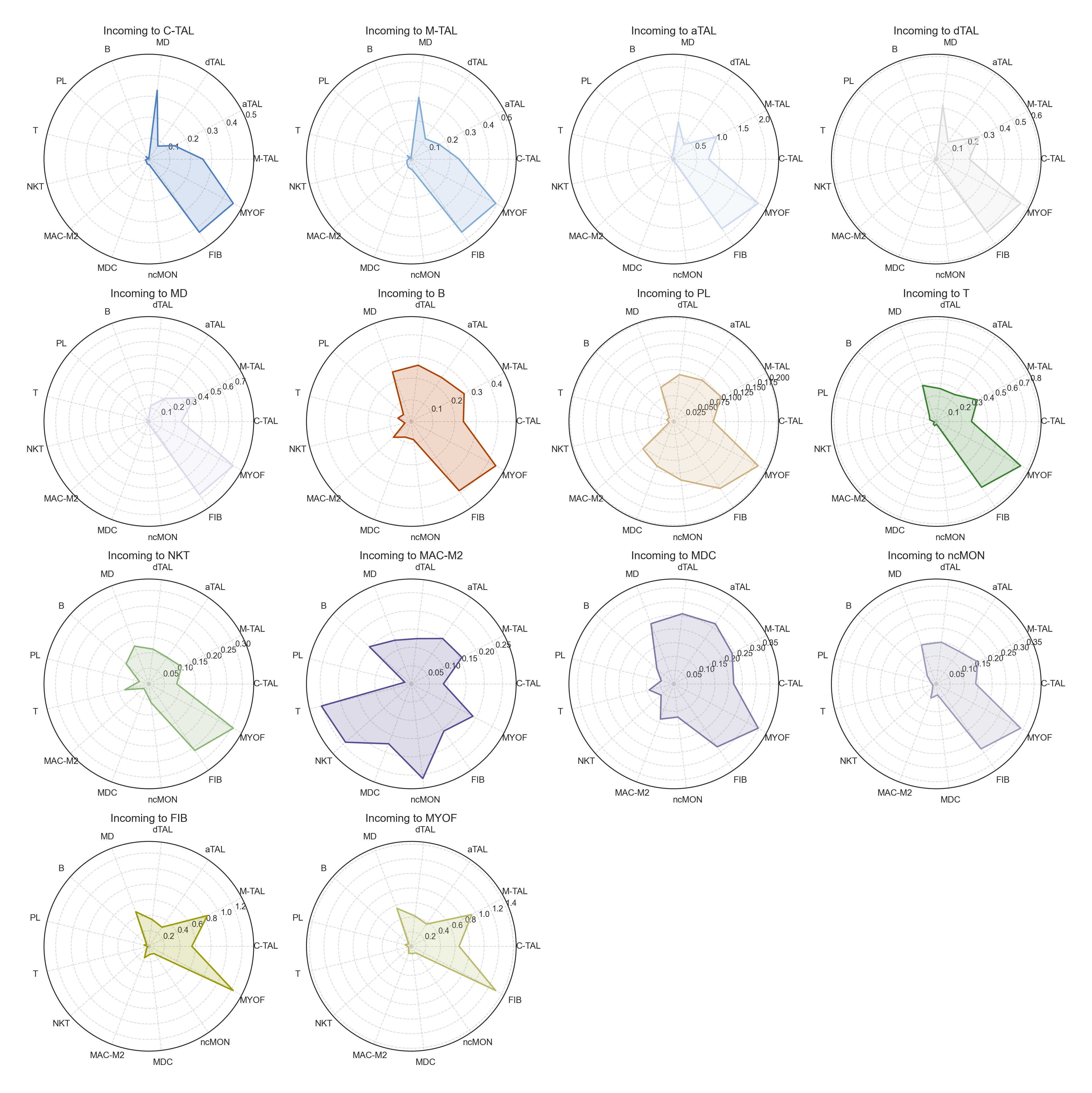
fig, ax = lvis.plot_radar(mode="incoming", kind="strength")
Intracellular Communication#
merged_df = scm.tl.infer_signal_pairs(
    gdata,
    meta_mdata,
    liana_res=cellchat_res,
    rtf_prior_net="combined_RTF",
    target_celltypes=["aTAL", "C-TAL", "M-TAL"],
)
INFO Starting Receptor-TF downstream analysis...
INFO Loading built-in RTF network: 'combined_RTF'
INFO Filtering prior network for 68 receptors and 54 TFs.
WARNING WARNING: 'dpt_pseudotime' not found in `meta_mdata`. Calculating from `data`...
INFO Ordering 107 metacells by 'dpt_pseudotime'.
INFO Calculating original scores for 834 R-T pairs.
INFO Performing permutation test with 1000 permutations...
INFO Calculating p-values and adjusting for multiple testing.
          Receptor-TF Downstream Analysis Summary
┏━━━━━━━━━━━━━━━━━━━━━━━━━━━━━━━━━━━━━━━━━━━━━━━━━┳━━━━━━━┓
┃                                          Metric ┃ Value ┃
┡━━━━━━━━━━━━━━━━━━━━━━━━━━━━━━━━━━━━━━━━━━━━━━━━━╇━━━━━━━┩
│                        Tested Receptor-TF pairs │ 834   │
│ Significant pairs (by covariance, adj p < 0.05) │ 301   │
└─────────────────────────────────────────────────┴───────┘
INFO Analysis complete.
source_celltypes = ["MAC-M2", "MDC", "ncMON", "NKT", "PL", "T", "B", "FIB", "MYOF"]
source_imm = ["MAC-M2", "MDC", "ncMON", "NKT", "PL", "T", "B"]
source_fib = ["FIB", "MYOF"]
merged_df_fil_imm = merged_df[
    (merged_df["pval_cov_adj"] < 0.01)
    & (merged_df["cellchat_pvals"] < 0.01)
    & (merged_df["source"].isin(source_imm))
    & (merged_df["target"] == "aTAL")
]


merged_df_fil_fib = merged_df[
    (merged_df["pval_cov_adj"] < 0.01)
    & (merged_df["cellchat_pvals"] < 0.01)
    & (merged_df["source"].isin(source_fib))
    & (merged_df["target"] == "aTAL")
]
merged_df_fil_imm
| signal_pairs | ligand_receptor | receptor | TF | dot_product | covariance | pval_dot | pval_cov | pval_dot_adj | pval_cov_adj | ... | ligand_props | ligand_trimean | mat_max | receptor_complex | receptor_props | receptor_trimean | source | target | lr_probs | cellchat_pvals | |
|---|---|---|---|---|---|---|---|---|---|---|---|---|---|---|---|---|---|---|---|---|---|
| 31 | SPP1-CD44-ZEB1 | SPP1-CD44 | CD44 | ZEB1 | 5.764141 | 1.262087 | 0.000999 | 0.000999 | 0.003967 | 0.003967 | ... | 0.403226 | 0.069604 | 7.855748 | CD44 | 0.398593 | 0.067263 | T | aTAL | 0.009277 | 0.0 |
| 32 | SPP1-CD44-ZEB1 | SPP1-CD44 | CD44 | ZEB1 | 5.764141 | 1.262087 | 0.000999 | 0.000999 | 0.003967 | 0.003967 | ... | 0.443750 | 0.064268 | 7.855748 | CD44 | 0.398593 | 0.067263 | MDC | aTAL | 0.008572 | 0.0 |
| 37 | SPP1-CD44-ZEB1 | SPP1-CD44 | CD44 | ZEB1 | 5.764141 | 1.262087 | 0.000999 | 0.000999 | 0.003967 | 0.003967 | ... | 0.376344 | 0.056561 | 7.855748 | CD44 | 0.398593 | 0.067263 | ncMON | aTAL | 0.007551 | 0.0 |
| 39 | SPP1-CD44-ZEB1 | SPP1-CD44 | CD44 | ZEB1 | 5.764141 | 1.262087 | 0.000999 | 0.000999 | 0.003967 | 0.003967 | ... | 0.366412 | 0.053767 | 7.855748 | CD44 | 0.398593 | 0.067263 | MAC-M2 | aTAL | 0.007181 | 0.0 |
| 40 | SPP1-CD44-ZEB1 | SPP1-CD44 | CD44 | ZEB1 | 5.764141 | 1.262087 | 0.000999 | 0.000999 | 0.003967 | 0.003967 | ... | 0.349131 | 0.052891 | 7.855748 | CD44 | 0.398593 | 0.067263 | B | aTAL | 0.007065 | 0.0 |
| ... | ... | ... | ... | ... | ... | ... | ... | ... | ... | ... | ... | ... | ... | ... | ... | ... | ... | ... | ... | ... | ... |
| 20400 | IGF1-IGF1R-PPARA | IGF1-IGF1R | IGF1R | PPARA | 18.289663 | 0.027069 | 0.000999 | 0.000999 | 0.003967 | 0.003967 | ... | 0.273092 | 0.028645 | 7.855748 | IGF1R | 0.623681 | 0.180689 | PL | aTAL | 0.010246 | 0.0 |
| 21523 | BMP6-BMPR1A-TCF7L2 | BMP6-BMPR1A | BMPR1A | TCF7L2 | 15.832006 | 0.021230 | 0.000999 | 0.000999 | 0.003967 | 0.003967 | ... | 0.253012 | 0.012410 | 7.855748 | BMPR1A_BMPR2 | 0.318875 | 0.037661 | PL | aTAL | 0.000934 | 0.0 |
| 21917 | IGF1-IGF1R-NFIA | IGF1-IGF1R | IGF1R | NFIA | 19.676503 | 0.021143 | 0.000999 | 0.000999 | 0.003967 | 0.003967 | ... | 0.273092 | 0.028645 | 7.855748 | IGF1R | 0.623681 | 0.180689 | PL | aTAL | 0.010246 | 0.0 |
| 22501 | IGF1-IGF1R-THRB | IGF1-IGF1R | IGF1R | THRB | 21.584236 | 0.015595 | 0.000999 | 0.000999 | 0.003967 | 0.003967 | ... | 0.273092 | 0.028645 | 7.855748 | IGF1R | 0.623681 | 0.180689 | PL | aTAL | 0.010246 | 0.0 |
| 22510 | IGF1-IGF1R-NFIC | IGF1-IGF1R | IGF1R | NFIC | 17.402330 | 0.015565 | 0.000999 | 0.000999 | 0.003967 | 0.003967 | ... | 0.273092 | 0.028645 | 7.855748 | IGF1R | 0.623681 | 0.180689 | PL | aTAL | 0.010246 | 0.0 |
350 rows × 22 columns
Visualization#
imm_tf_list = merged_df_fil_imm["TF"].value_counts()[merged_df_fil_imm["TF"].value_counts() > 10].index.tolist()
fib_tf_list = merged_df_fil_fib["TF"].value_counts()[merged_df_fil_fib["TF"].value_counts() > 10].index.tolist()

union_tf_list = list(set(imm_tf_list) | set(fib_tf_list))
union_tf_list
['KLF5',
 'MBD2',
 'ELF3',
 'NR4A1',
 'ZEB1',
 'TCF12',
 'NFE2L2',
 'ETS1',
 'TEAD1',
 'JUN',
 'STAT3',
 'RUNX1',
 'EPAS1',
 'SMAD3',
 'SOX4',
 'KLF6',
 'EGR1',
 'HIF1A']
scm.pl.stripplot(
    gdata,
    sortby="degree_centrality",
    n_top=30,
    selected_genes=union_tf_list,
)
imm_receptor_list = (
    merged_df_fil_imm["receptor"].value_counts()[merged_df_fil_imm["receptor"].value_counts() > 10].index.tolist()
)
fib_receptor_list = (
    merged_df_fil_fib["receptor"].value_counts()[merged_df_fil_fib["receptor"].value_counts() > 10].index.tolist()
)

union_receptor_list = list(set(imm_receptor_list) | set(fib_receptor_list))
union_receptor_list
['ITGAV', 'FGFR1', 'CD44', 'ITGB1', 'SDC4', 'ITGA3', 'INSR', 'MET', 'ITGA6']
imm_ligand_list = (
    merged_df_fil_imm["ligand"].value_counts()[merged_df_fil_imm["ligand"].value_counts() > 10].index.tolist()
)
fib_ligand_list = (
    merged_df_fil_fib["ligand"].value_counts()[merged_df_fil_fib["ligand"].value_counts() > 10].index.tolist()
)

union_ligand_list = list(set(imm_ligand_list) | set(fib_ligand_list))
union_ligand_list
['COL1A1',
 'COL6A2',
 'COL6A1',
 'COL6A3',
 'FN1',
 'LAMA4',
 'NCAM1',
 'THBS1',
 'LAMC3',
 'COL4A4',
 'LAMA2',
 'COL4A1',
 'HGF',
 'NAMPT',
 'LAMC1',
 'COL4A5',
 'COL1A2',
 'SPP1',
 'COL4A3',
 'COL4A2',
 'LAMB1',
 'LAMA3']
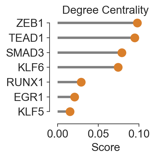
tf_list = ["TEAD1", "ZEB1", "KLF6", "SMAD3", "EGR1", "KLF5", "RUNX1"]
receptor_list = ["CD44", "ITGAV", "ITGA3", "ITGA6", "ITGB8", "SDC4", "FGFR1"]
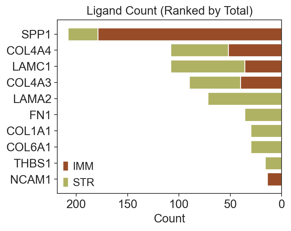
ligand_list = ["SPP1", "COL1A1", "COL6A1", "COL4A3", "COL4A4", "LAMC1", "LAMA2", "FN1", "THBS1", "NCAM1"]
tf_score = gdata["GRN"].varm["network_score"].copy()
sns.set_style("ticks")

lollipop_plot_df = tf_score.loc[tf_list].copy()
lollipop_plot_df = lollipop_plot_df.sort_values(by="degree_centrality", ascending=False)
sorted_tf_list = lollipop_plot_df.index.tolist()

tf_names = lollipop_plot_df.index[::-1].tolist()
scores = lollipop_plot_df["degree_centrality"].values[::-1]

fig, ax = plt.subplots(figsize=(3, 3))

ax.hlines(y=tf_names, xmin=0, xmax=scores, color="gray", linewidth=3)

ax.plot(scores, tf_names, "o", color="#D97F2B", markersize=10)

ax.set_xlabel("Score")
ax.set_xlim(0, max(scores) + 0.02)
ax.set_title("Degree Centrality")

sns.despine(offset=10, trim=True)
plt.tight_layout()
imm_counts_df = merged_df_fil_imm["ligand"].value_counts()
str_counts_df = merged_df_fil_fib["ligand"].value_counts()

counts_df = pd.concat([imm_counts_df, str_counts_df], axis=1)
counts_df.columns = ["IMM", "STR"]


filtered_df = counts_df.reindex(ligand_list).fillna(0)
filtered_df["Total"] = filtered_df["IMM"] + filtered_df["STR"]
sorted_df = filtered_df.sort_values(by="Total", ascending=False)
sorted_ligand_list = sorted_df.index.tolist()

fig, ax = plt.subplots(figsize=(5, 4))
y_pos = range(len(sorted_df.index))

ax.barh(y_pos, sorted_df["IMM"], color="#984D28", label="IMM")
ax.barh(y_pos, sorted_df["STR"], left=sorted_df["IMM"], color="#B0B263", label="STR")


ax.set_yticks(y_pos)
ax.set_yticklabels(sorted_df.index)
ax.invert_yaxis()
ax.invert_xaxis()
ax.set_xlabel("Count")
ax.set_title("Ligand Count (Ranked by Total)")
ax.legend()

plt.tight_layout()
plt.show()
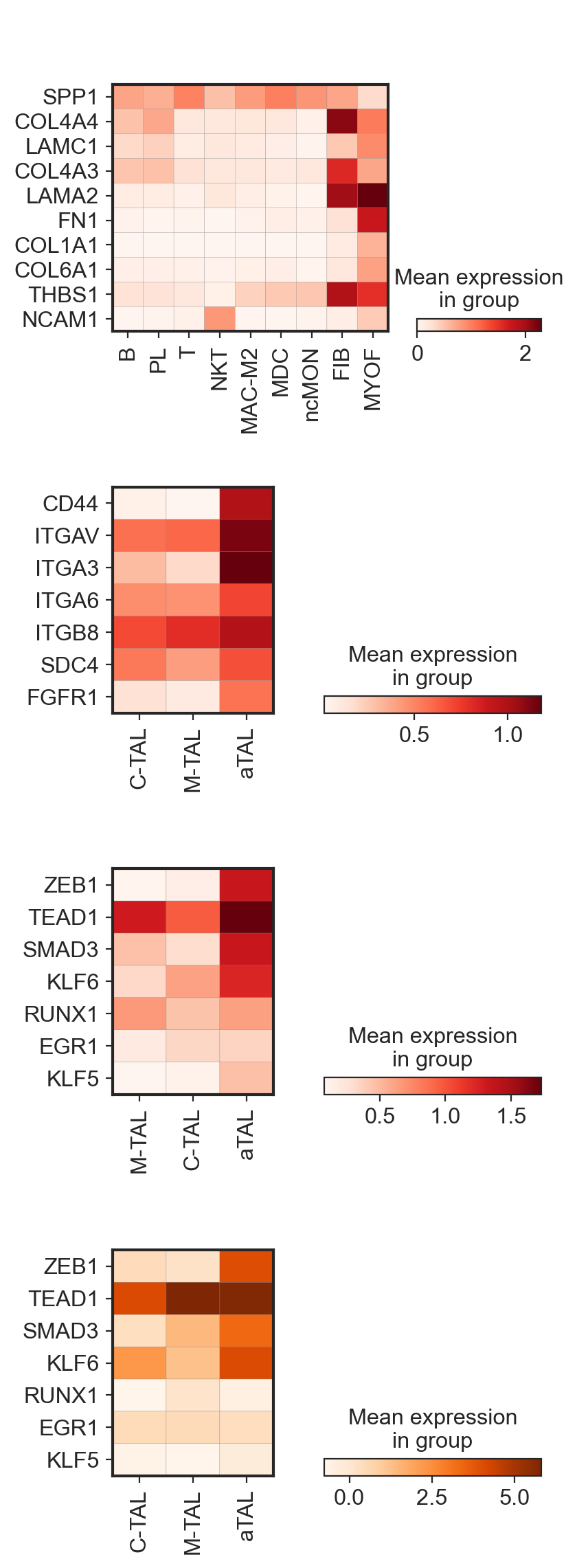
fig, ax = plt.subplots(4, 1, figsize=(4, 14))

sc.pl.matrixplot(
    adata_cci[~(adata_cci.obs["subclass.l1"] == "TAL")],
    var_names=sorted_ligand_list,
    groupby="celltype",
    cmap="Reds",
    swap_axes=True,
    show=False,
    ax=ax[0],
    use_raw=False,
)

sc.pl.matrixplot(
    adata_cci[(adata_cci.obs["subclass.l1"] == "TAL") & (adata_cci.obs["celltype"].isin(["C-TAL", "M-TAL", "aTAL"]))],
    var_names=receptor_list,
    groupby="celltype",
    cmap="Reds",
    swap_axes=True,
    show=False,
    ax=ax[1],
    use_raw=False,
)

sc.pl.matrixplot(
    gdata["RNA"],
    layer="log1p_norm",
    var_names=sorted_tf_list,
    groupby="celltype",
    cmap="Reds",
    swap_axes=True,
    show=False,
    ax=ax[2],
    use_raw=False,
)

sc.pl.matrixplot(
    gdata["GRN"], var_names=sorted_tf_list, groupby="celltype", cmap="Oranges", swap_axes=True, ax=ax[3], use_raw=False
)
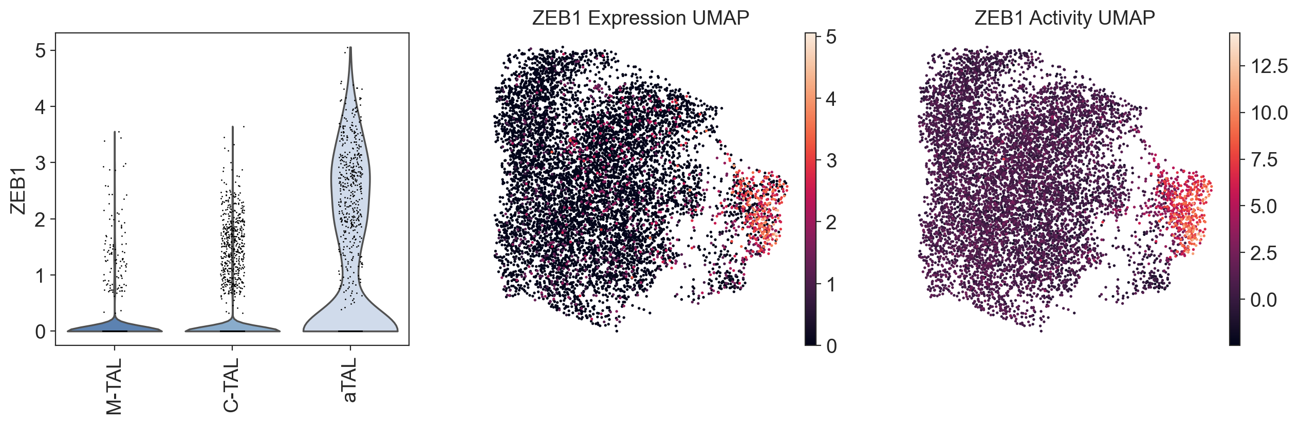
tf = "ZEB1"
fig, ax = plt.subplots(1, 3, figsize=(15, 4))
sc.pl.violin(gdata["RNA"], tf, groupby="celltype", rotation=90, layer="log1p_norm", use_raw=False, ax=ax[0], show=False)
sc.pl.umap(gdata["RNA"], color=tf, use_raw=False, frameon=False, ax=ax[1], show=False, title=f"{tf} Expression UMAP")
sc.pl.umap(gdata["GRN"], color=tf, use_raw=False, frameon=False, ax=ax[2], show=True, title=f"{tf} Activity UMAP")
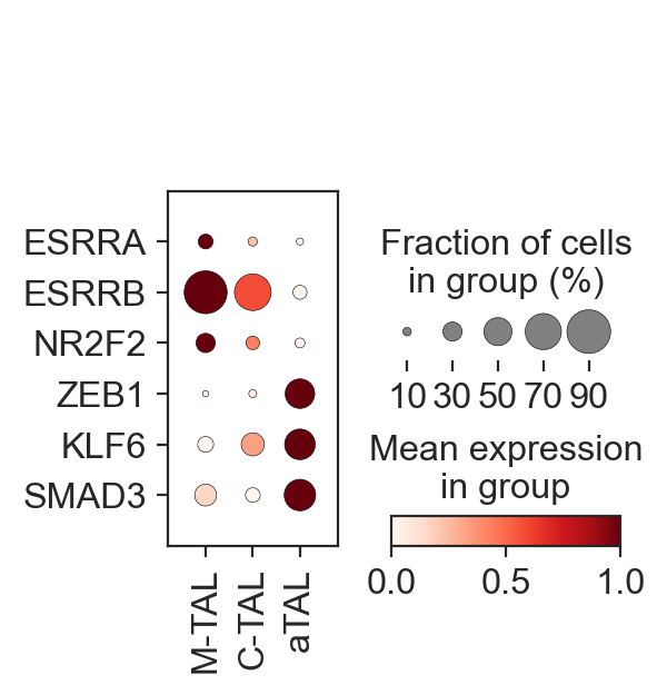
sc.pl.dotplot(
    gdata["RNA"],
    var_names=["ESRRA", "ESRRB", "NR2F2", "ZEB1", "KLF6", "SMAD3"],
    groupby="celltype",
    standard_scale="var",
    cmap="Reds",
    swap_axes=True,
)
sns.set_style("ticks")
scm.pl.trendplot(
    gdata,
    var_dict={
        "TEAD1": ["RNA"],
        "ZEB1": ["RNA"],
        "KLF6": ["RNA"],
        "SMAD3": ["RNA"],
        "ESRRA": ["RNA"],
        "ESRRB": ["RNA"],
        "NR2F2": ["RNA"],
    },
    normalize=True,
    sortby="dpt_pseudotime",
    col_color=["celltype"],
    figsize=(6.5, 3),
    n_splines=4,
    show_tkey=False,
    swap_x=False,
    show_stds=False,
)
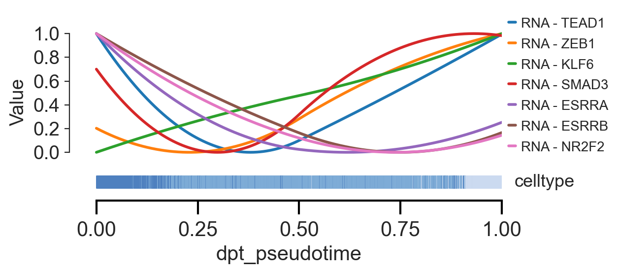
<Axes: xlabel='dpt_pseudotime', ylabel='Value'>
filtered_df = merged_df[
    (merged_df["ligand"].isin(sorted_ligand_list))
    & (merged_df["receptor"].isin(receptor_list))
    & (merged_df["TF"].isin(sorted_tf_list))
    & (merged_df["source"].isin(source_celltypes))
    & (merged_df["target"] == "aTAL")
]


lr_agg_df = (
    filtered_df.groupby(["ligand", "receptor"])
    .agg(lr_probs=("lr_probs", "sum"))
    .reset_index()
    .sort_values(by="lr_probs", ascending=False)
)
rtf_agg_df = (
    filtered_df.groupby(["receptor", "TF"])
    .agg(rtf_covs=("covariance", "mean"))
    .reset_index()
    .sort_values(by="rtf_covs", ascending=False)
)
celltype_order = ["M-TAL", "C-TAL", "aTAL"]
gdata["RNA"].obs["celltype"] = pd.Categorical(gdata["RNA"].obs["celltype"], categories=celltype_order, ordered=True)
gdata["GRN"].obs["celltype"] = pd.Categorical(gdata["GRN"].obs["celltype"], categories=celltype_order, ordered=True)
celltype_order = [
    "M-TAL",
    "C-TAL",
    "aTAL",
    "dTAL",
    "MD",
    "B",
    "PL",
    "T",
    "NKT",
    "MAC-M2",
    "MDC",
    "ncMON",
    "FIB",
    "MYOF",
]
adata_cci.obs["celltype"] = pd.Categorical(adata_cci.obs["celltype"], categories=celltype_order, ordered=True)
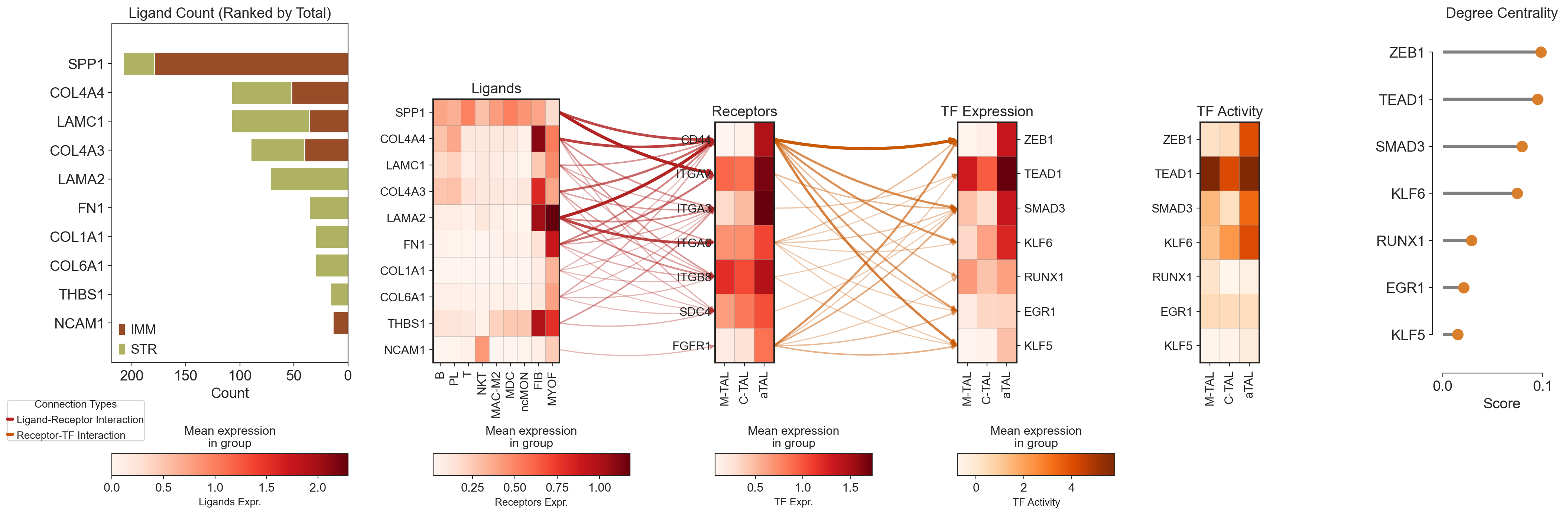
# Import necessary libraries
from matplotlib.patches import ConnectionPatch
import matplotlib.gridspec as gridspec
from matplotlib.lines import Line2D

# --- Assume these data objects are already loaded in your environment ---
# adata_cci = ...
# gdata = ...
# sorted_ligand_list = ['SPP1', ...]  # Example gene
# receptor_list = ['CD44', ...]     # Example gene
# sorted_tf_list = ['STAT3', ...]      # Example TF

# =============================================================================
# 1. Setup a custom figure layout for THREE plots
# =============================================================================
# Create the main figure (the "canvas"), making it wider for three plots
fig = plt.figure(figsize=(25, 8))

# Define a 2-row, 3-COLUMN grid. The top row for plots is much taller.
gs = gridspec.GridSpec(2, 6, wspace=0.5, hspace=0.5, width_ratios=[6, 5, 4, 4, 4, 3], height_ratios=[15, 1])

# Create three axes for the main plots in the top row
axes = [
    fig.add_subplot(gs[0, 0]),
    fig.add_subplot(gs[0, 1]),
    fig.add_subplot(gs[0, 2]),
    fig.add_subplot(gs[0, 3]),
    fig.add_subplot(gs[0, 4]),
    fig.add_subplot(gs[0, 5]),
]

# ax_tf_activity = axes[3]
# ax_lollipop = fig.add_subplot(gs[0, 4])
# axes.append(ax_lollipop)
ax_ligand_barh = axes[0]
ax_lollipop = axes[5]

legend_axes = [
    fig.add_subplot(gs[1, 0]),
    fig.add_subplot(gs[1, 1]),
    fig.add_subplot(gs[1, 2]),
    fig.add_subplot(gs[1, 3]),
]

# =============================================================================
# 2. Draw the three matrixplots
# =============================================================================

# Plot 0: Ligand count barplot

filtered_df = counts_df.reindex(ligand_list).fillna(0)
filtered_df["Total"] = filtered_df["IMM"] + filtered_df["STR"]
sorted_df = filtered_df.sort_values(by="Total", ascending=False)
sorted_ligand_list = sorted_df.index.tolist()

y_pos = range(len(sorted_df.index))
ax_ligand_barh.barh(y_pos, sorted_df["IMM"], color="#984D28", label="IMM")
ax_ligand_barh.barh(y_pos, sorted_df["STR"], left=sorted_df["IMM"], color="#B0B263", label="STR")
ax_ligand_barh.set_yticks(y_pos)
ax_ligand_barh.set_yticklabels(sorted_df.index)
ax_ligand_barh.invert_yaxis()
ax_ligand_barh.invert_xaxis()
ax_ligand_barh.set_xlabel("Count")
ax_ligand_barh.set_title("Ligand Count (Ranked by Total)")
ax_ligand_barh.legend()
# Remove y-axis labels from the first plot for a cleaner look
ax_ligand_barh.set_ylabel("")
ax_ligand_barh.margins(y=0.1)

# --- Plot 1: Ligands ---
plot_dict_ligand = sc.pl.matrixplot(
    adata_cci[~(adata_cci.obs["subclass.l1"] == "TAL")],
    var_names=sorted_ligand_list,
    groupby="celltype",
    cmap="Reds",
    swap_axes=True,
    show=False,
    ax=axes[1],
    use_raw=False,
)
ax_ligand = plot_dict_ligand["mainplot_ax"]
ax_ligand.set_title("Ligands")
# Remove y-axis labels from the first plot for a cleaner look
ax_ligand.set_ylabel("")

# --- Plot 2: Receptors ---
plot_dict_receptor = sc.pl.matrixplot(
    adata_cci[(adata_cci.obs["subclass.l1"] == "TAL") & (adata_cci.obs["celltype"].isin(["M-TAL", "C-TAL", "aTAL"]))],
    var_names=receptor_list,
    groupby="celltype",
    cmap="Reds",  # Changed cmap for visual distinction
    swap_axes=True,
    show=False,
    ax=axes[2],
    use_raw=False,
)
ax_receptor = plot_dict_receptor["mainplot_ax"]
ax_receptor.set_title("Receptors")
# Remove y-axis labels and ticks from the middle plot
ax_receptor.set_ylabel("")
ax_receptor.tick_params(axis="y", length=0)


# --- Plot 3: Transcription Factors (TF) Expression---
plot_dict_tf = sc.pl.matrixplot(
    gdata["RNA"],
    layer="log1p_norm",
    var_names=sorted_tf_list,
    groupby="celltype",
    cmap="Reds",  # Changed cmap for visual distinction
    swap_axes=True,
    show=False,
    ax=axes[3],
    use_raw=False,
)
ax_tf = plot_dict_tf["mainplot_ax"]
ax_tf.set_title("TF Expression")
# Move the y-axis labels of the last plot to the right
ax_tf.yaxis.tick_right()
ax_tf.yaxis.set_label_position("right")


# --- Plot 4: TF Activity ---
plot_dict_tf_activity = sc.pl.matrixplot(
    gdata["GRN"],
    var_names=sorted_tf_list,
    groupby="celltype",
    cmap="Oranges",  # Changed cmap for visual distinction
    swap_axes=True,
    show=False,
    ax=axes[4],
    use_raw=False,
)

ax_tf_activity = plot_dict_tf_activity["mainplot_ax"]
ax_tf_activity.set_title("TF Activity")


# --- Plot 5: Lollipop Plot for TF Degree Centrality ---
# Reuse the previously created lollipop plot axis
# lollipop_plot_df = gdata["GRN"].varm["network_score"].loc[sorted_tf_list].copy()
tf_names = lollipop_plot_df.index[::-1].tolist()
scores = lollipop_plot_df["degree_centrality"].values[::-1]
ax_lollipop.hlines(y=tf_names, xmin=0, xmax=scores, color="gray", linewidth=3)
ax_lollipop.plot(scores, tf_names, "o", color="#D97F2B", markersize=10)
ax_lollipop.set_xlabel("Score")
ax_lollipop.set_xlim(0, max(scores) + 0.02)
ax_lollipop.set_title("Degree Centrality")

sns.despine(ax=ax_lollipop, offset=10, trim=True)
ax_lollipop.margins(y=0.1)
# sns.despine(offset=10, trim=True)
# plt.setp(ax_lollipop.get_yticklabels(), visible=False)  # Hide y-tick labels


# =============================================================================
# 3. Remove all individual color legends
# =============================================================================
# plot_dict_ligand['color_legend_ax'].remove()
# plot_dict_receptor['color_legend_ax'].remove()
# plot_dict_tf['color_legend_ax'].remove()
# plot_dict_tf_activity['color_legend_ax'].remove()

# =============================================================================
# 4. Add connection arrows between plots
# =============================================================================
lr_color = "#B22222"
rtf_color = "#C95902"


# =============================================================================
# 1. Normalization Function
# =============================================================================
# A helper function to scale a series of values to a new range (e.g., for line width or alpha)
def normalize_for_plot(series, min_val, max_val):
    """min-max scaling"""
    return min_val + (max_val - min_val) * (series - series.min()) / (series.max() - series.min())


# Normalize your data
lr_agg_df["linewidth"] = normalize_for_plot(lr_agg_df["lr_probs"], 1.0, 3.0)  # Line width from 0.5 to 4.0
lr_agg_df["alpha"] = normalize_for_plot(lr_agg_df["lr_probs"], 0.3, 1.0)  # Alpha from 0.3 to 1.0

rtf_agg_df["linewidth"] = normalize_for_plot(rtf_agg_df["rtf_covs"], 1.0, 3.0)
rtf_agg_df["alpha"] = normalize_for_plot(rtf_agg_df["rtf_covs"], 0.3, 1.0)


# --- Draw Ligand -> Receptor connections ---
# Get the actual y-tick labels (gene names) from the plot axes
ligand_plot_genes = [label.get_text() for label in ax_ligand.get_yticklabels()]
receptor_plot_genes = [label.get_text() for label in ax_receptor.get_yticklabels()]

for _, row in lr_agg_df.iterrows():
    # Check if both ligand and receptor are present in the plots
    if row["ligand"] in ligand_plot_genes and row["receptor"] in receptor_plot_genes:
        # Get coordinates
        y_start = ligand_plot_genes.index(row["ligand"]) + 0.5
        y_end = receptor_plot_genes.index(row["receptor"]) + 0.5
        x_start = len(ax_ligand.get_xticklabels())
        x_end = 0

        # Create the patch with scaled properties
        con = ConnectionPatch(
            xyA=(x_start, y_start),
            xyB=(x_end, y_end),
            coordsA="data",
            coordsB="data",
            axesA=ax_ligand,
            axesB=ax_receptor,
            arrowstyle="-|>",  # Simple line, no arrowhead
            linewidth=row["linewidth"],
            color=lr_color,
            alpha=row["alpha"],  # Use scaled alpha for color depth
            connectionstyle="arc3,rad=0.1",
            zorder=10,
        )
        fig.add_artist(con)


# --- Draw Receptor -> TF connections ---
tf_plot_genes = [label.get_text() for label in ax_tf.get_yticklabels()]

for _, row in rtf_agg_df.iterrows():
    if row["receptor"] in receptor_plot_genes and row["TF"] in tf_plot_genes:
        y_start = receptor_plot_genes.index(row["receptor"]) + 0.5
        y_end = tf_plot_genes.index(row["TF"]) + 0.5
        x_start = len(ax_receptor.get_xticklabels())
        x_end = 0

        con = ConnectionPatch(
            xyA=(x_start, y_start),
            xyB=(x_end, y_end),
            coordsA="data",
            coordsB="data",
            axesA=ax_receptor,
            axesB=ax_tf,
            arrowstyle="-|>",
            linewidth=row["linewidth"],
            color=rtf_color,
            alpha=row["alpha"],
            mutation_scale=10,
            connectionstyle="arc3,rad=0.1",
            zorder=10,
        )
        fig.add_artist(con)

# ============================================================================
# 5. Plot color legends
# ============================================================================


# --- Legend 1 for Ligands ---
# Get the original legend axes
orig_legend_ax1 = plot_dict_ligand["color_legend_ax"]
# Get the new position from the placeholder axes we created
new_pos1 = legend_axes[0].get_position()
# Apply the new position to the original legend axes
orig_legend_ax1.set_position(new_pos1)
# Reorient the legend to be horizontal
orig_legend_ax1.xaxis.set_ticks_position("bottom")
orig_legend_ax1.xaxis.set_label_position("bottom")
orig_legend_ax1.set_xlabel("Ligands Expr.", fontsize=10)  # Add a label
# Remove the placeholder axes
legend_axes[0].remove()


# --- Legend 2 for Receptors ---
orig_legend_ax2 = plot_dict_receptor["color_legend_ax"]
new_pos2 = legend_axes[1].get_position()
orig_legend_ax2.set_position(new_pos2)
orig_legend_ax2.xaxis.set_ticks_position("bottom")
orig_legend_ax2.xaxis.set_label_position("bottom")
orig_legend_ax2.set_xlabel("Receptors Expr.", fontsize=10)
legend_axes[1].remove()


# --- Legend 3 for TF Expression ---
orig_legend_ax3 = plot_dict_tf["color_legend_ax"]
new_pos3 = legend_axes[2].get_position()
orig_legend_ax3.set_position(new_pos3)
orig_legend_ax3.xaxis.set_ticks_position("bottom")
orig_legend_ax3.xaxis.set_label_position("bottom")
orig_legend_ax3.set_xlabel("TF Expr.", fontsize=10)
legend_axes[2].remove()


# --- Legend 4 for TF Activity ---
orig_legend_ax4 = plot_dict_tf_activity["color_legend_ax"]
new_pos4 = legend_axes[3].get_position()
orig_legend_ax4.set_position(new_pos4)
orig_legend_ax4.xaxis.set_ticks_position("bottom")
orig_legend_ax4.xaxis.set_label_position("bottom")
orig_legend_ax4.set_xlabel("TF Activity", fontsize=10)
legend_axes[3].remove()


legend_handles = [
    Line2D([0], [0], color=lr_color, lw=3, label="Ligand-Receptor Interaction"),
    Line2D([0], [0], color=rtf_color, lw=3, label="Receptor-TF Interaction"),
]

# Add the legend to the figure. 'loc' determines the position.
# 'bbox_to_anchor' allows for fine-tuning the position.
fig.legend(
    handles=legend_handles,
    loc="lower right",  # Position the legend in the bottom-left corner
    bbox_to_anchor=(0.2, 0.2),  # Fine-tune position (x, y) in figure coordinates
    fontsize=10,
    frameon=True,  # Add a frame around the legend
    title="Connection Types",
)

# =============================================================================
# 5. Show the final plot
# =============================================================================
plt.show()
scm.pl.trendplot(
    gdata,
    var_dict={"CD44": ["RNA"], "FGFR1": ["RNA"], "ZEB1": ["RNA", "GRN"]},
    normalize=True,
    sortby="dpt_pseudotime",
    col_color=["celltype"],
    figsize=(6.5, 3),
    n_splines=5,
    show_tkey=False,
    swap_x=False,
    show_stds=False,
)
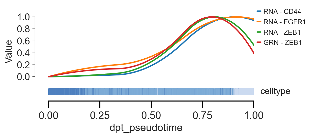
<Axes: xlabel='dpt_pseudotime', ylabel='Value'>